Skyborn Typhoon Maximum Potential Intensity

Prologue: An Ordinary GitHub Issue

Hello, Would it be possible to add a function to compute tropical cyclone (TC) potential intensity (PI) in Skyborn? PI is a widely used variable in the TC community. It defines the theoretical maximum intensity of a tropical cyclone in a given environment as defined by temperature and humidity. The only existing Python package to compute it (Gilford et al., 2021) is a Python translation of K. Emanuel’s Matlab code, it is not built in a very flexible manner, does not handle units well and is very slow.

Recently, I received an email from a GitHub issue stating that tcpypi’s computation speed is too slow and it does not handle variable units well.

Time flies, and by the time I wrote this post, it had been exactly one year since the last post about computing Typhoon GPI, Python | Typhoon GPI | Potential Intensity.

Meanwhile, Typhoon “Tabah” has made landfall in Guangdong.

Upon rereading the tcpypi documentation, I found that it takes 27 minutes to compute global potential intensity (PI) data at a 0.25° resolution for a year!

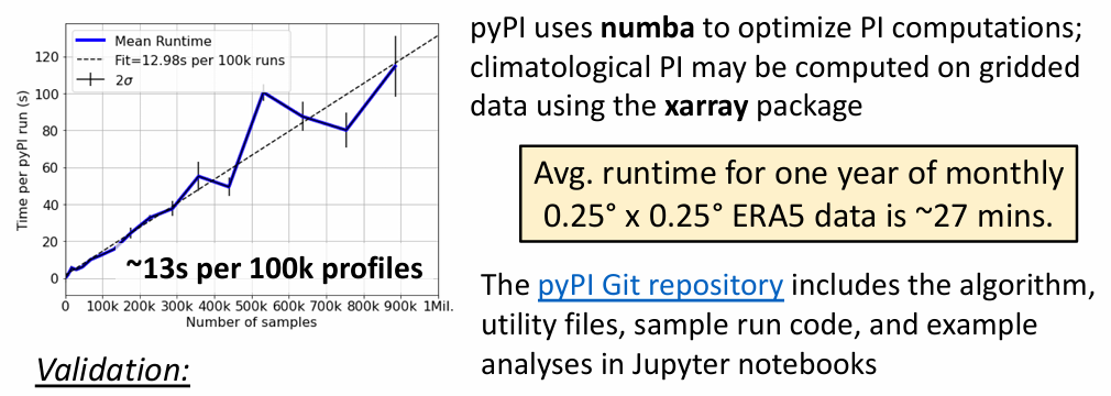
In climate research, it is often necessary to process decades of high-resolution data. If you have to wait nearly half an hour every year, then a 30-year climate state analysis would take 15 hours! Such an efficiency bottleneck severely restricts research progress.

Today, I bring a solution—Skyborn’s GPI submodule will completely change this situation.

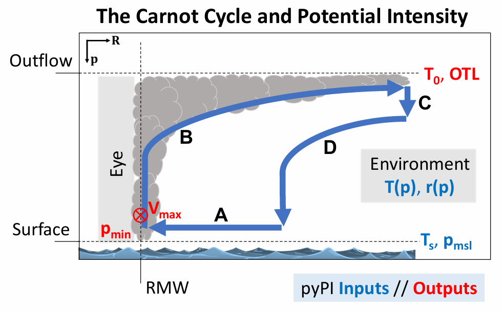
First Movement: Transition from Point to Area

The traditional tcpypi uses a point-by-point loop calculation method, like a diligent craftsman building a wall brick by brick:

# Traditional method of tcpyPI: point-by-point loop
for y in range(nlat):
    for x in range(nlon):
        if sst[y, x] > 0:
            result = pi(sst[y, x], msl[y, x], pressure,
                       temp[:, y, x], q[:, y, x], ...)
            vmax[y, x] = result[0]
            pmin[y, x] = result[1]

This method, while intuitive, is known to be a performance killer when performing large loops in Python.

Skyborn adopts a completely new approach—whole array processing:

# Modern method of Skyborn: whole array computation
from skyborn.calc.GPI.xarray import potential_intensity

# Directly process the entire array without manual loops
min_pressure, max_wind, error = potential_intensity(
    sst,              # (nlat, nlon)
    psl,              # (nlat, nlon)  
    pressure_levels,  # (nlevels,)
    temperature,      # (nlevels, nlat, nlon)
    mixing_ratio      # (nlevels, nlat, nlon)
)

The interface is simple and elegant, and a single function call can complete all calculations without the need for additional for loops.

Second Movement: Intelligent Unit Conversion—Returning Science to Its Essence

In actual research, data sources have a variety of units:

• ERA5 gives you Kelvin and hPa
• CMIP6 data may be in Kelvin and Pascals
• Observation data follows another set of standards

tcpyPI requires users to handle all unit conversions themselves, and a slight oversight can lead to errors. Skyborn has a built-in intelligent unit recognition and conversion system:

# Skyborn automatically handles common units
import xarray as xr
from skyborn.calc.GPI.xarray import potential_intensity

# Directly pass in xarray data with unit attributes
ds = xr.open_dataset('ERA5_data.nc')

# Automatically recognize and convert units
result = potential_intensity(
    sst=ds.sst,           # Automatically recognized: °C → K
    psl=ds.msl,           # Automatically recognized: hPa → Pa
    pressure_levels=ds.level,
    temperature=ds.t,      # Automatically recognized: °C → K
    mixing_ratio=ds.q      # Automatically recognized: g/kg → kg/kg
)

Third Movement: Performance Leap—19 to 25 Times Speedup

Let’s let the data speak. Under the same hardware conditions, processing the global sample data provided by tcpypi:

Benchmark Results

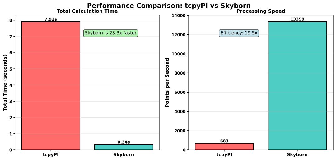
The speed of Skyborn computing PI is 19-25 times that of tcpypi.

This means that computations that originally required overnight runs can now be completed in the time it takes to have a meal or go for a 5-kilometer run! (Of course, this does not consider the time required to read the data.)

Validation of Computation Results

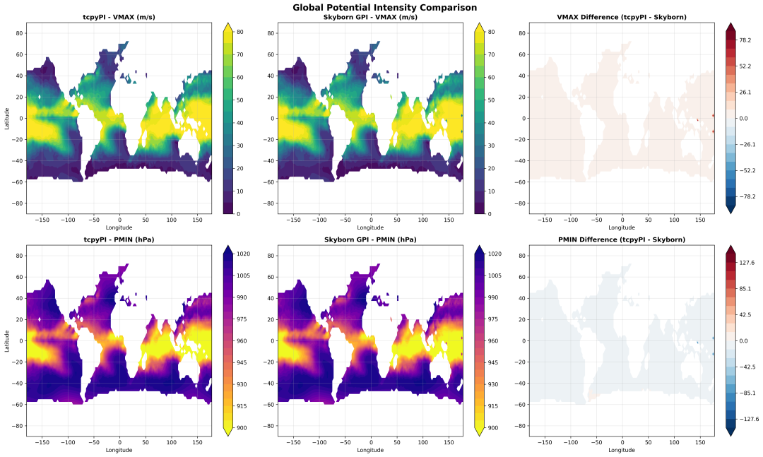
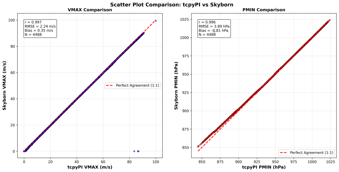
It can be seen that there are only a few outliers, with a correlation coefficient of 0.996, indicating that the computation results are quite close.

Fourth Movement: User Guide—Details Determine Success or Failure

When using Skyborn to compute PI, there are several key points that need special attention:

1. It is recommended to use the xarray interface

Skyborn provides two interfaces: numpy array interface and xarray interface. It is strongly recommended to use the xarray interface, as it can automatically handle unit conversions and dimension management:

from skyborn.calc.GPI.xarray import potential_intensity
import xarray as xr

# Load data
ds = xr.open_dataset('your_data.nc')

# Use xarray interface - recommended way!
result = potential_intensity(
    sst=ds.sst,
    psl=ds.msl,
    pressure_levels=ds.level,
    temperature=ds.t,
    mixing_ratio=ds.q
)

2. Unit attributes are crucial

The intelligent unit conversion of Skyborn relies on correct unit attributes.Be sure to add the correct unit attributes to the data:

# Correctly set unit attributes - this step is very important!
sst_da.attrs['units'] = 'degrees C'  # or 'K' 
psl_da.attrs['units'] = 'hPa'        # or 'Pa'
temp_da.attrs['units'] = 'degrees C'  # or 'K'
mixr_da.attrs['units'] = 'g/kg'      # or 'kg/kg'

# Skyborn will automatically recognize and convert these units

Supported unit formats:

• Temperature: <span>'degrees C'</span>, <span>'degC'</span>, <span>'celsius'</span>, <span>'K'</span>, <span>'kelvin'</span>
• Pressure: <span>'hPa'</span>, <span>'mb'</span>, <span>'Pa'</span>, <span>'pascal'</span>
• Mixing Ratio: <span>'g/kg'</span>, <span>'kg/kg'</span>, <span>'1'</span> (dimensionless)

3. Pressure level order

Skyborn will automatically handle the ordering of pressure levels, but it is important to understand how it works:

# Pressure levels can be in any order
pressure_levels = [1000, 925, 850, 700, 500, 300, 200, 100]  # from ground to high altitude
# or
pressure_levels = [100, 200, 300, 500, 700, 850, 925, 1000]  # from high altitude to ground

# Skyborn will automatically adjust to the required order

4. Handling missing values

Skyborn automatically detects and intelligently handles missing values, but the missing values in nc data generated by ncl have not been tested, so it is recommended to use pure Python for reading and processing.

5. Dimension requirements

Ensure that the data dimensions match correctly:

# 1D data (single vertical profile)
sst              # scalar value
psl              # scalar value
temperature.shape # (nlevels,)
mixing_ratio.shape # (nlevels,)

# 3D data (spatial field at a single time)
sst.shape        # (nlat, nlon)
psl.shape        # (nlat, nlon)
temperature.shape # (nlevels, nlat, nlon)
mixing_ratio.shape # (nlevels, nlat, nlon)

# 4D data (time series)
sst.shape        # (ntime, nlat, nlon)
psl.shape        # (ntime, nlat, nlon)
temperature.shape # (ntime, nlevels, nlat, nlon)
mixing_ratio.shape # (ntime, nlevels, nlat, nlon)

6. Example: Calculating PI with ERA5 data

import xarray as xr
from skyborn.calc.GPI.xarray import potential_intensity

# 1. Load ERA5 data
ds = xr.open_dataset('ERA5_2023_08.nc')

# 2. Check and set unit attributes
# ERA5 usually uses K and Pa, but it's best to confirm
print(f"SST units: {ds.sst.attrs.get('units', 'unknown')}")
print(f"MSL units: {ds.msl.attrs.get('units', 'unknown')}")

# 3. Ensure unit attributes are correct
if 'units' not in ds.sst.attrs:
    ds.sst.attrs['units'] = 'K'  # ERA5 defaults to Kelvin
if 'units' not in ds.msl.attrs:
    ds.msl.attrs['units'] = 'Pa'  # ERA5 defaults to Pascals
if 'units' not in ds.t.attrs:
    ds.t.attrs['units'] = 'K'
if 'units' not in ds.q.attrs:
    ds.q.attrs['units'] = 'kg/kg'  # ERA5 defaults to kg/kg

# 4. Calculate PI
result = potential_intensity(
    sst=ds.sst,
    psl=ds.msl,
    pressure_levels=ds.level,  # ERA5 pressure level variable
    temperature=ds.t,
    mixing_ratio=ds.q
)

# 5. The result contains two variables
print(f"Maximum wind speed: {result.pi}")  # Potential Intensity (m/s)
print(f"Minimum pressure: {result.min_pressure}")  # Minimum pressure (hPa)

7. Common Issues and Precautions

Vertical Level Count is Crucial

# Important reminder: The number of vertical levels may affect calculation accuracy!

# Not recommended: Too few levels
pressure_levels = [1000, 850, 500, 200]  # Only 4 levels, poor accuracy

# Recommended: Sufficient vertical resolution
pressure_levels = [1000, 975, 950, 925, 900, 850, 800, 750, 
                  700, 650, 600, 550, 500, 450, 400, 350,
                  300, 250, 200, 150, 100, 70, 50]  # 23 levels

# ERA5 standard 37 levels or ERA5.1's 137 levels are ideal choices

Recommendations:

• Use at least 10 pressure levels
• Ideally use more than 20 levels
• Ensure to include boundary layer details (1000-850 hPa)
• Ensure to extend to the top of the troposphere (at least to 100 hPa)

Other Common Issues

1. Missing or Incorrect Unit Attributes

• Symptoms: Abnormal results (e.g., PI > 200 m/s or < 10 m/s)
• Causes: Data units do not match expectations
• Solutions: Clearly set unit attributes, such as <span>ds.sst.attrs['units'] = 'K'</span>

2. Missing Key Pressure Levels

• Symptoms: Inaccurate CAPE calculations, low PI values
• Causes: Insufficient vertical resolution, try to increase vertical resolution as much as possible
• Solutions: Ensure data includes near-surface layers (1000, 975, 950 hPa, etc.)

3. Confusion in Mixing Ratio Units

• Symptoms: Errors in humidity-related calculations
• Causes: Misusing relative humidity instead of mixing ratio
• Solutions: Skyborn requires mixing ratio (mixing ratio) which is specific humidity q, not relative humidity (RH)!

Fifth Movement: Installation and Usage

System Requirements:

• Python Version: 3.9 – 3.13
• Operating System: Windows (x64), macOS (Intel/Apple Silicon), Linux (x86_64)

To install the Skyborn library, you can use pip:

pip install skyborn

Or use the following command:

pip install -U --index-url https://pypi.org/simple/ skyborn

Conclusion

A year ago, I introduced the basic concepts of GPI and PI.

Today, Skyborn has transformed these theories into efficient computational tools.

Acknowledgments

Thanks to the user who raised the valuable issue. It is your feedback that drives this project forward.

Special thanks to Professor Kerry Emanuel for his pioneering work on PI theory, which has laid a solid foundation for typhoon research.

Related Links

❝

• Skyborn Documentation: https://skyborn.readthedocs.io/en/latest/
• GitHub Repository: https://github.com/QianyeSu/Skyborn

Previous Reviews

• Python | Typhoon GPI | Potential Intensity
• Python | Spherical Harmonics | Stream Function | Potential Function
• Python | Skyborn | Missing Value Filling

References

[1] Emanuel, K. A. (1988): The maximum intensity of hurricanes. Journal of the Atmospheric Sciences, 45(7), 1143-1155.

[2] Emanuel, K. A. (1995): Sensitivity of tropical cyclones to surface exchange coefficients and a revised steady-state model incorporating eye dynamics. Journal of the Atmospheric Sciences, 52(22), 3969-3976.

[3] Bister, M., & Emanuel, K. A. (1998): Dissipative heating and hurricane intensity. Meteorology and Atmospheric Physics, 65(3-4), 233-240. https://doi.org/10.1007/BF01030791

[4] Bister, M., & Emanuel, K. A. (2002): Low frequency variability of tropical cyclone potential intensity 1. Interannual to interdecadal variability. Journal of Geophysical Research: Atmospheres, 107(D24), 4801. https://doi.org/10.1029/2001JD000776

[5] Emanuel, K., & Nolan, D. S. (2004): Tropical cyclone activity and the global climate system. Bulletin of the American Meteorological Society, 85(5), 666-667.

[6] Emanuel, K. (2005): Increasing destructiveness of tropical cyclones over the past 30 years. Nature, 436(7051), 686-688. https://doi.org/10.1038/nature03906

[7] Gilford, D. M. (2021): pyPI (v1.3): Tropical Cyclone Potential Intensity Calculations in Python. Geoscientific Model Development, 14(5), 2351-2369. https://doi.org/10.5194/gmd-14-2351-2021