Introduction to the Python Statistics Module

For small statistical analyses, there is really no need to install a bunch of large libraries. If you want to calculate an average or check the distribution of sales data, you might end up spending a lot of time installing pandas, numpy, etc., and by then, your enthusiasm might have cooled down.

In fact, the built-in <span>statistics</span> module in Python can handle most daily statistical needs: calculating means, finding medians, checking distributions, and playing with normal curves; it has everything you need.

1. The “Heart” of Data — Measures of Central Tendency

When describing the core characteristics of a dataset, the first thing that comes to mind is where its “center” is. Central tendency is the metric that measures the central position of data, telling us what the most typical value of the data is.<span>statistics</span> module provides a wealth of tools for this purpose.

1.1 The Mean Family: More Than Just “Average”

Calculating the mean seems simple, but its meaning and calculation method can vary greatly in different contexts.<span>statistics</span> thoughtfully provides a series of functions known as the “mean family” to meet various needs.

<span>mean()</span> vs. <span>fmean()</span>: The Choice Between Speed and Precision

The most common average is the arithmetic mean, which is the sum of all data points divided by the number of data points.

<span>statistics</span> module provides two functions to achieve this: <span>mean()</span> and <span>fmean()</span>.

• <span>mean()</span>: A general-purpose, high-precision arithmetic mean function.
• <span>fmean()</span>: A faster arithmetic mean function specifically for handling floating-point numbers, which always returns a <span>float</span>.

Why is <span>mean()</span> slower than <span>fmean()</span>?

Beginners may wonder why there are two functions that seem so similar.

★

<span>mean()</span> is not slow due to “implementation differences”; rather, it is designed to maintain robustness and preserve type semantics across different numeric types (including <span>Decimal</span>/<span>Fraction</span>). It uses a more robust but slower summation strategy internally; <span>fmean()</span> converts everything to float and uses high-precision floating-point summation, making it faster in pure floating-point scenarios, with sufficient precision, but it loses the semantics of <span>Decimal</span>/<span>Fraction</span> and always returns a <span>float</span>.

<span>geometric_mean()</span>: A Tool for Calculating Average Growth Rates

When you need to calculate the “average” of a series of percentage changes (like return on investment or population growth rates), the arithmetic mean can be misleading. This is because these changes are multiplicative rather than additive. In this case, you should use the geometric mean.

Its calculation method is to multiply all values (which must be positive) and then take the n-th root, where n is the number of values. The formula is:.

Practical Example: Return on Investment

Suppose an investment grows by 50% in the first year (becoming 1.5 times its original value), and then loses 50% in the second year (becoming half its value, or 0.5 times).

import statistics

# Growth factors corresponding to the growth rates
growth_factors = [1.5, 0.5]

# Incorrect calculation: using arithmetic mean
# (1.5 + 0.5) / 2 = 1.0, which means an average growth rate of 0%, which is clearly wrong
# Because an investment of 100 will become 100 * 1.5 * 0.5 = 75, which is actually a loss
arithmetic_avg_factor = statistics.mean(growth_factors)
print(f"Arithmetic average growth factor: {arithmetic_avg_factor:.4f}")
print(f"Final value based on arithmetic average (100): {100 * arithmetic_avg_factor * arithmetic_avg_factor:.2f}\n")

# Correct calculation: using geometric mean
# sqrt(1.5 * 0.5) = sqrt(0.75) ≈ 0.866
# This means the average value becomes 0.866 times its original value each year, indicating an average annual loss of 13.4%
geometric_avg_factor = statistics.geometric_mean(growth_factors)
print(f"Geometric average growth factor: {geometric_avg_factor:.4f}")
print(f"Final value based on geometric average (100): {100 * geometric_avg_factor * geometric_avg_factor:.2f}")

# Output
Arithmetic average growth factor: 1.0000
Final value based on arithmetic average (100): 100.00

Geometric average growth factor: 0.8660
Final value based on geometric average (100): 75.00

<span>harmonic_mean()</span>: The Ultimate Solution for Average Rate Problems

The harmonic mean is another special type of mean that is suitable for calculating averages of rates, such as speed (km/h).

Its calculation method is: the number of data points divided by the sum of the reciprocals of all data points. The formula is:.

Practical Example: Average Speed

A classic problem is: you drive to a city at a speed of 60 km/h, and return at a speed of 40 km/h. What is the average speed for the entire trip?

Many people would intuitively use the arithmetic mean <span>(60 + 40) / 2 = 50</span> km/h, but this is incorrect. Because you spend more time driving slowly at 40 km/h, the slower speed should have a greater weight. The harmonic mean perfectly solves this problem.

import statistics

speeds =  # km/h

# Incorrect calculation: using arithmetic mean
arithmetic_avg_speed = statistics.mean(speeds)
print(f"Arithmetic average speed: {arithmetic_avg_speed} km/h\n")

# Correct calculation: using harmonic mean
# Assuming distance is D. Time to go = D/60, time to return = D/40.
# Total distance = 2D, total time = D/60 + D/40.
# Average speed = total distance / total time = 2D / (D/60 + D/40) = 2 / (1/60 + 1/40) = 48 km/h
harmonic_avg_speed = statistics.harmonic_mean(speeds)
print(f"Harmonic average speed: {harmonic_avg_speed} km/h")

# Output
Arithmetic average speed: 50 km/h

Harmonic average speed: 48.0 km/h

Comparison of Mean Functions

Function Name	Main Application Scenario	Supported Data Types	Key Features
<span>mean()</span>	General arithmetic mean	<span>int</span>, <span>float</span>, <span>Decimal</span>, <span>Fraction</span>	High precision, can handle special numeric types, slightly slower
<span>fmean()</span>	Fast calculation for regular floating-point/integer	<span>int</span>, <span>float</span> (internally converted to <span>float</span>)	Fast, always returns <span>float</span>
<span>geometric_mean()</span>	Average growth rates, return rates, etc. for multiplicative sequences	Positive numbers	Correctly reflects compound growth
<span>harmonic_mean()</span>	Average rates, ratios, etc.	Positive numbers	Correctly handles average rates, giving more weight to smaller values

1.2 Median: Finding the Most Stable Center Point

The median is the value that lies in the middle of a sorted dataset. Compared to the mean, its greatest advantage is its insensitivity to outliers, meaning it has robustness.

For example, for the dataset <span>[1, 2, 3, 4, 100]</span>, the mean is <span>22</span> (severely inflated by the outlier <span>100</span>), while the median is <span>3</span>, which better represents the “typical” central position of this dataset.

<span>statistics</span> module provides three functions related to the median, with differences in how they handle even numbers of data points.

• <span>median()</span>: Standard median. If the number of data points is even, it returns the arithmetic mean of the two middle numbers.
• <span>median_low()</span>: Low median. If the number of data points is even, it returns the smaller of the two middle numbers.
• <span>median_high()</span>: High median. If the number of data points is even, it returns the larger of the two middle numbers.

import statistics

# When the number of data points is odd, all three results are the same
data_odd = [1, 3, 5]
print(f"Odd dataset: {data_odd}")
print(f"median(): {statistics.median(data_odd)}")
print(f"median_low(): {statistics.median_low(data_odd)}")
print(f"median_high(): {statistics.median_high(data_odd)}\n")

# When the number of data points is even, the three results differ
data_even = [1, 3, 5, 7]
print(f"Even dataset: {data_even}")
# The two middle numbers are 3 and 5
print(f"median(): {statistics.median(data_even)}") # (3+5)/2 = 4.0
print(f"median_low(): {statistics.median_low(data_even)}") # Returns 3
print(f"median_high(): {statistics.median_high(data_even)}") # Returns 5

# Output
Odd dataset: [1, 3, 5]
median(): 3
median_low(): 3
median_high(): 3

Even dataset: [1, 3, 5, 7]
median(): 4.0
median_low(): 3
median_high(): 5

Common Pitfall: Using <span>median()</span> on Discrete Data

Imagine you are analyzing discrete ratings from 1 to 5 stars (which can only take integer values). If the dataset is <span>[1, 2, 3, 4]</span>, <span>median()</span> will return <span>2.5</span> — but your system does not have a “2.5 star”. In this case, using <span>median_low()</span> or <span>median_high()</span> is more appropriate: they guarantee to return values that actually appear in the data, which are 2 (more conservative) or 3 (more optimistic). Choosing between <span>low</span> or <span>high</span> depends on your business preference.

1.3 Mode: Discovering the “High-Frequency Words” in Data

The mode is the value that appears most frequently in a dataset, commonly used for categorical data (like colors, brands) and discrete values (like ratings, ages).

<span>mode()</span> vs <span>multimode()</span>:

• <span>mode(data)</span> : Returns the most common single value.
• Python 3.7 and earlier: If there are multiple modes (like <span>[1, 2, 1, 2]</span>), it will raise a <span>StatisticsError</span>.
• Python 3.8+: If there are ties, it returns the first mode that appears in the data (the above example returns <span>1</span>).
• <span>multimode(data)</span> (3.8+) : Returns a list of all modes; when there are ties, the results are given in the order of their first appearance in the original data (e.g., <span>[2, 1, 2, 1, 3, 3]</span> → <span>[2, 1, 3]</span>).

Common Pitfalls

• Need to robustly handle ties: Prefer using <span>multimode()</span>; if your business can only accept one value, then establish your own decision rules for ties (like taking the first, the maximum, the minimum, etc.).
• Empty Data: <span>mode([])</span> will raise an error; <span>multimode([])</span> returns an empty list. Check before calling or prefer using <span>multimode()</span> for peace of mind.
• Do not assume result order: The return order of <span>multimode()</span> is related to the first appearance order, not the numerical size.

import statistics
import sys

# Check Python version
print(f"Current Python version: {sys.version}\n")

data_single_mode = ['red', 'blue', 'blue', 'red', 'green', 'red', 'red']
# Make '2' and '3' have the same frequency, with '2' appearing first in the sequence
data_multi_mode  = ['2', '3', '2', '3', '1']

# Single mode case
print(f"Single mode data: {data_single_mode}")
print(f"mode(): {statistics.mode(data_single_mode)}")
print(f"multimode(): {statistics.multimode(data_single_mode)}\n")

# Multiple modes case
print(f"Multiple mode data: {data_multi_mode}")
# In Python 3.8+, mode() returns the first encountered mode '2'
print(f"mode(): {statistics.mode(data_multi_mode)}")
# multimode() returns all modes ['2', '3'] (in the order of first appearance)
print(f"multimode(): {statistics.multimode(data_multi_mode)}")

# Output
Current Python version: 3.11.3 (tags/v3.11.3:f3909b8, Apr  4 2023, 23:49:59) [MSC v.1934 64 bit (AMD64)]

Single mode data: ['red', 'blue', 'blue', 'red', 'green', 'red', 'red']
mode(): red
multimode(): ['red']

Multiple mode data: ['2', '3', '2', '3', '1']
mode(): 2
multimode(): ['2', '3']

2. The “Fat and Thin” of Data — Measures of Dispersion

Is the data tightly clustered around the mean, or is it widely dispersed? This is the question that measures of spread aim to answer.

Variance and Standard Deviation: How to Choose the Most Suitable Function?

Variance and standard deviation quantify “how much fluctuation there is”.Standard deviation is the square root of variance, and its unit is the same as the original data, making it easier to intuitively understand.

In the <span>statistics</span> module, there are two pairs of corresponding APIs, and you need to first determine whether your data is a “population” or a “sample”:

• Sample (if you want to use this part of the data to infer a larger population) use <span>variance()</span> / <span>stdev()</span>. They use n−1 (Bessel’s correction) internally to avoid underestimating the population variance.
• Population (if you only care about the entire batch of data you have) use <span>pvariance()</span> / <span>pstdev()</span><span>, where the denominator is </span><strong><span>N</span></strong><span>.</span>

★

One sentence to remember:Sample → <span>variance/stdev</span> (n−1), Population → <span>pvariance/pstdev</span> (N). You don’t need to derive the formula; Bessel’s correction is already handled by <span>statistics</span>.

import statistics as stats

# 5 heights (cm) sampled from a larger population
heights = [168, 172, 171, 169, 175]  # n = 5

# Treating as a population (denominator N)
print("Population variance:", round(stats.pvariance(heights), 2))
print("Population standard deviation:", round(stats.pstdev(heights), 2))

# Treating as a sample (denominator n-1, Bessel's correction applied)
print("Sample variance:", round(stats.variance(heights), 2))
print("Sample standard deviation:", round(stats.stdev(heights), 2))

# Output
Population variance: 6
Population standard deviation: 2.45
Sample variance: 7.5
Sample standard deviation: 2.74

You will see:Sample variance/standard deviation is generally slightly larger than the population’s — this is a reasonable upward adjustment due to the n−1 correction, which avoids underestimating overall fluctuations.

Common Pitfalls

<span>variance()</span> / <span>stdev()</span> requires at least 2 samples, otherwise it raises a <span>StatisticsError</span>; <span>pvariance()</span> / <span>pstdev()</span> will return <span>0</span> for a single data point.

Quick Reference Table

Statistic	Population Function (denominator N)	Sample Function (denominator n−1)	Typical Scenario
Variance	<span>pvariance()</span>	<span>variance()</span>	Describing full data vs. sampling estimation
Standard Deviation	<span>pstdev()</span>	<span>stdev()</span>	Describing full data vs. sampling estimation

★

Practical Guide: First ask yourself“Is what I have the whole or just a part?” Most data analysis is sample, so prefer using <span>variance()</span> / <span>stdev()</span>; only when you truly have all the data and want to describe it itself, use <span>pvariance()</span> / <span>pstdev()</span><span>.</span>

3. Delving into Data Distribution

3.1 <span>quantiles()</span><code><span>: The "Cutting Master" of Data Distribution</span>

Quantiles divide the sorted data into several equal parts, using cut points to describe the distribution position. Common names include:

• Quartiles (Q1, Q2, Q3) divide the data into 4 parts;
• Deciles divide the data into 10 parts;
• Percentiles divide the data into 100 parts.

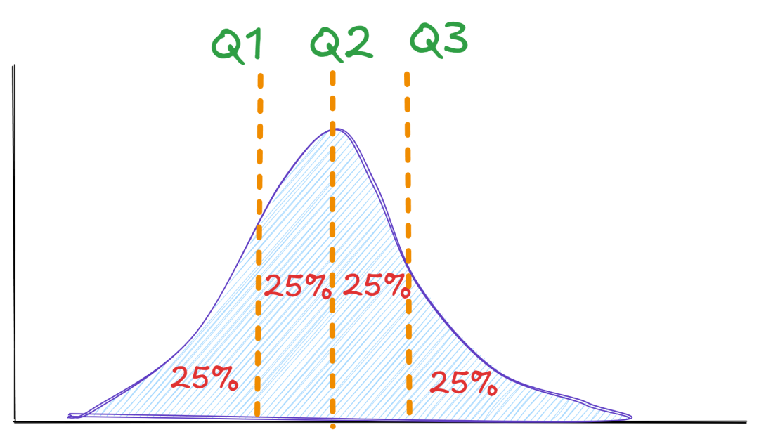
<span>statistics.quantiles()</span> is used to calculate these cut points, returning a list of length <span>n-1</span> (excluding the minimum and maximum values):

# No need for pre-sorting, the function will sort automatically
statistics.quantiles(data, *, n=4, method='exclusive')

• <span>n</span>: The number of parts to divide into (default is 4, i.e., quartiles, returning 3 cut points).
• <span>method</span>: <span>'exclusive'</span> (default) or <span>'inclusive'</span>, used to control the interpolation method.

How to Choose <span>method</span>

• Sample Data (more common): Use the default <span>method='exclusive'</span>, as this is how quantiles are commonly calculated in statistics.

• Need to ensure that quantiles definitely fall within the range [minimum, maximum] (small samples/displaying more conservatively): Use <span>method='inclusive'</span>. For very small datasets, <span>exclusive</span> may give quantiles that slightly exceed the extreme values (due to interpolation characteristics), while <span>inclusive</span> will be “constrained” within the extreme value range.

  import statistics as stats
  
  # Example 1: Only two data points
  data = [0, 10]
  print("Extreme value range:", min(data), "～", max(data))
  print("exclusive quartiles:", stats.quantiles(data, n=4, method='exclusive'))
  print("inclusive quartiles:", stats.quantiles(data, n=4, method='inclusive'))
  
  

  # Output
  Extreme value range: 0 ～ 10
  exclusive quartiles: [-2.5, 5.0, 12.5]
  inclusive quartiles: [2.5, 5.0, 7.5]
  

★

The differences between the two methods mainly manifest in small samples; the larger the sample, the less noticeable the difference.

Example: Quartiles and Deciles

import statistics as stats

# Exam scores of 20 students (sample)
scores = [78, 82, 84, 85, 86, 87, 88, 89, 90, 91,
          91, 92, 93, 94, 95, 95, 96, 97, 98, 100]

# Quartiles (Q1, Q2=Median, Q3), default method='exclusive'
q = stats.quantiles(scores, n=4)
print("Quartiles (Q1, Q2=Median, Q3):", [round(x, 2) for x in q])

# Deciles (returns 9 cut points)
d = stats.quantiles(scores, n=10)   # Default is still 'exclusive'
print("Deciles:", [round(x, 2) for x in d])

# If you want quartiles to strictly fall within the extreme values, you can choose:
q_inclusive = stats.quantiles(scores, n=4, method='inclusive')
print("Quartiles (inclusive):", [round(x, 2) for x in q_inclusive])

# Output
Quartiles (Q1, Q2=Median, Q3): [86.25, 91.0, 95.0]
Deciles: [82.2, 85.2, 87.3, 89.4, 91.0, 92.6, 94.7, 95.8, 97.9]
Quartiles (inclusive): [86.75, 91.0, 95.0]

How to Interpret?<span>quantiles(scores, n=4)</span><code><span> returns the three position points Q1, Q2 (median), Q3. For example, the "middle 50%" of the data roughly falls between </span><code><span>[Q1, Q3]</span><span>, which is the </span><strong><span>IQR</span></strong><span> (interquartile range).</span>

Common Pitfalls

• <span>quantiles()</span> requires at least 2 data points; for very small samples, <span>exclusive</span> may give quantiles that slightly exceed the extreme values, so use <span>inclusive</span> for a more conservative approach.
• The results may be non-integer values/not present in the original data — because interpolation is used.
• The return is cut points rather than intervals; to describe “how much data falls within which quantile range”, you need to combine with counting/histograms.

3.2 Visualization: Using Box Plots to “See Through” Distribution

Box plots clearly convey the “five-number summary” of the data: minimum, first quartile (Q1), median (Q2), third quartile (Q3), and maximum; they also mark points that exceed the “whisker” range as outliers.

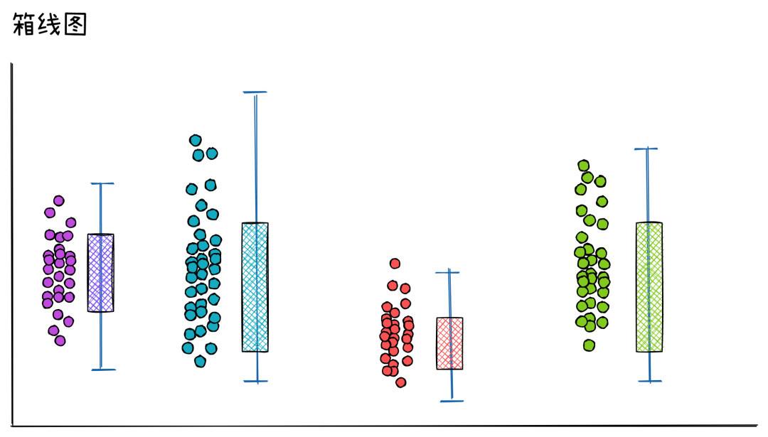
How to Quickly Understand Box Plots

• Box: Lower edge = Q1, upper edge = Q3; box height = IQR = Q3 − Q1, the thicker the box, the more dispersed the middle 50% of the data.
• Median Line: The horizontal line inside the box = Q2 (median).
• Whiskers: Usually extend to the minimum/maximum observations within the range of <span>Q1 − 1.5*IQR</span> and <span>Q3 + 1.5*IQR</span>.
• Outliers: Points that fall outside the whiskers.

Example: Same Mean, Different Dispersion

import statistics as stats
import numpy as np
import matplotlib.pyplot as plt

# Simulate two groups of scores: same mean, but different dispersion
np.random.seed(42)
scores_A = np.random.normal(loc=85, scale=5,  size=100)   # Small fluctuation
scores_B = np.random.normal(loc=85, scale=15, size=100)   # Large fluctuation

# Calculate quartiles (showing how to use statistics to get quantiles)
qA = stats.quantiles(scores_A, n=4)  # [Q1, Q2, Q3]
qB = stats.quantiles(scores_B, n=4)
print(f"Class A: Q1={qA[0]:.2f}, Median={qA[1]:.2f}, Q3={qA[2]:.2f}")
print(f"Class B: Q1={qB[0]:.2f}, Median={qB[1]:.2f}, Q3={qB[2]:.2f}")

# Draw box plots (side-by-side comparison of the two distributions)
fig, ax = plt.subplots(figsize=(8, 6))
ax.boxplot([scores_A, scores_B], labels=["Class A", "Class B"], showfliers=True)

ax.set_title("Comparison of Class A and B Score Distributions (Same Mean, Different Dispersion)")
ax.set_ylabel("Scores")
ax.yaxis.grid(True)

plt.show()

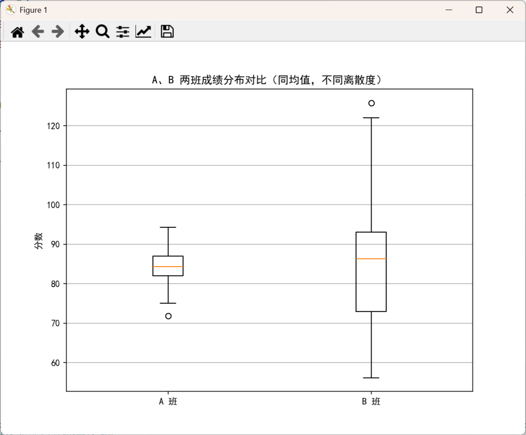
Chart Interpretation

• Class A: The box is narrower, and the whiskers are shorter → the distribution is more concentrated, and stability is better.
• Class B: The box is wider, and the whiskers are longer → greater differences, higher dispersion, and outliers are more likely to occur.

Without looking at the raw data, just by looking at one chart, you can quickly judge “who is more stable, how much difference there is, and whether there are outliers” — this is the value of quantiles and box plots.

4. The Magic of Normal Distribution — <span>NormalDist</span> Object

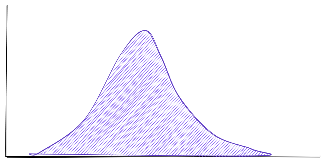
Normal distribution, also known as Gaussian distribution, is one of the most common probability distributions in nature and human society. From height, weight to exam scores and measurement errors, countless phenomena approximately follow a normal distribution. The <span>NormalDist</span> object introduced in Python 3.8 provides extremely convenient tools for handling calculations related to normal distribution.

4.1 Creating and Using <span>NormalDist</span>

<span>NormalDist</span> objects encapsulate two core parameters of a normal distribution: mean (<span>mu</span>) and standard deviation (<span>sigma</span>). They can be created in two ways, corresponding to the two core modes of statistical work:from theoretical modeling and from observational modeling.

• <span>NormalDist(mu, sigma)</span>: Create from known theoretical parameters

  When you already know that a phenomenon follows a normal distribution and are clear about its mean and standard deviation, you can use this constructor.

• <span>NormalDist.from_samples(data)</span>: Estimate parameters from sample data and create

  When you only have a bunch of raw data and want to fit or describe it with a normal distribution, this class method will automatically calculate the sample mean and sample standard deviation from the data, then create a NormalDist object.

import statistics

# Method 1: Create from theoretical parameters
# Assume we know that the height of adult males in a certain area follows a normal distribution with a mean of 175cm and a standard deviation of 6cm
height_dist_theoretical = statistics.NormalDist(mu=175, sigma=6)
print(f"Theoretical model: {height_dist_theoretical}")

# Method 2: Create from sample data
# Assume we randomly measured the heights of 10 people
height_samples = [170, 172, 168, 180, 175, 178, 177, 169, 174, 176]
height_dist_from_data = statistics.NormalDist.from_samples(height_samples)
print(f"Model estimated from sample data: {height_dist_from_data}")

# Output
Theoretical model: NormalDist(mu=175.0, sigma=6.0)
Model estimated from sample data: NormalDist(mu=173.9, sigma=4.04007700696685)

4.2 Probability Calculations and Threshold Searches (<span>pdf</span>, <span>cdf</span>, <span>inv_cdf</span>)

<span>NormalDist</span> objects are powerful because they provide a complete set of methods to answer various questions about probabilities.

“What is the likelihood of a specific value occurring?” — <span>pdf(x)</span>

<span>pdf(x)</span> (Probability Density Function) returns the probability density at the point <span>x</span>. It is important to note that for continuous distributions, the probability of a single point is zero, so the value of <span>pdf</span> itself is not a probability, but it reflects the relative likelihood around that point.<span>pdf</span> values that are larger indicate that the data is denser around those points.

“What is the probability of getting a value less than or equal to X?” — <span>cdf(x)</span>

<span>cdf(x)</span> (Cumulative Distribution Function) calculates the cumulative probability that a random variable is less than or equal to <span>x</span><span>, i.e., P(X≤x). This geometrically equals the area under the normal curve from negative infinity to </span><code><span>x</span><span>.</span><strong><span>Calculating the percentile of a value</span></strong><span> is a typical application of </span><code><span>cdf</span>.

“What score do I need to reach the top P%?” — <span>inv_cdf(p)</span>

<span>inv_cdf(p)</span> (Inverse Cumulative Distribution Function) is the inverse function of <span>cdf</span>, also known as the quantile function. You give it a probability <span>p</span> (between 0 and 1), and it returns the corresponding value <span>x</span>.

Practical Example: Analyzing SAT Scores

Assume that SAT exam scores follow a normal distribution with a mean of 1060 and a standard deviation of 195.

import statistics

# Create a normal distribution object for SAT scores
sat_dist = statistics.NormalDist(mu=1060, sigma=195)

# Question 1: What is the probability density for a randomly selected student whose score is around 1200?
pdf_1200 = sat_dist.pdf(1200)
print(f"Probability density at 1200: {pdf_1200:.6f}\n")

# Question 2: What is the probability that a randomly selected student scores below 1300?
# This is equivalent to calculating the percentile corresponding to 1300
prob_below_1300 = sat_dist.cdf(1300)
print(f"Probability of scoring below 1300: {prob_below_1300:.4f} (i.e., at the {prob_below_1300:.2%} percentile)\n")

# Question 3: What is the probability that a randomly selected student scores above 1300?
prob_above_1300 = 1 - sat_dist.cdf(1300)
print(f"Probability of scoring above 1300: {prob_above_1300:.4f}\n")

# Question 4: What is the minimum score needed to exceed 90% of students?
# This is equivalent to finding the score corresponding to the 90th percentile
score_top_10_percent = sat_dist.inv_cdf(0.90)
print(f"Minimum score required to be in the top 10% (i.e., exceeding 90% of people): {score_top_10_percent:.2f}")

# Output
Probability density at 1200: 0.001581

Probability of scoring below 1300: 0.8908 (i.e., at the 89.08% percentile)

Probability of scoring above 1300: 0.1092

Minimum score required to be in the top 10% (i.e., exceeding 90% of people): 1309.90

4.3 Histograms and Normal Curves

Is our data truly normally distributed? An intuitive way to test this is to plot the histogram of the data alongside its fitted normal distribution curve to see if they match.

We will generate a set of simulated data, then use <span>NormalDist.from_samples()</span> to create a model and compare it with the histogram of the original data.

import statistics
import matplotlib.pyplot as plt
import numpy as np

# Set Chinese font
plt.rcParams['font.sans-serif'] = ['SimHei']
plt.rcParams['axes.unicode_minus'] = False

# 1. Generate a set of approximately normally distributed sample data
np.random.seed(0)
sample_data = np.random.normal(loc=100, scale=15, size=500)

# 2. Create NormalDist object from sample data

dist_model = statistics.NormalDist.from_samples(sample_data)
mu = dist_model.mean
sigma = dist_model.stdev
print(f"Estimated mean (mu) from data: {mu:.2f}")
print(f"Estimated standard deviation (sigma) from data: {sigma:.2f}")

# 3. Draw histogram
# Key parameter: density=True. This normalizes the area of the histogram to 1, allowing direct comparison with the probability density function (PDF) curve
plt.figure(figsize=(10, 6))
plt.hist(sample_data, bins=30, density=True, alpha=0.6, color='g', label='Data Histogram')

# 4. Draw the fitted normal distribution PDF curve
# Create x-axis range for plotting the curve
xmin, xmax = plt.xlim()
x = np.linspace(xmin, xmax, 100)
# Calculate the PDF value for each x point
p = [dist_model.pdf(val) for val in x]
plt.plot(x, p, 'k', linewidth=2, label='Fitted Normal Distribution Curve')

# 5. Add chart elements

title = f"Data Distribution and Normal Fit (μ = {mu:.2f}, σ = {sigma:.2f})"
plt.title(title)
plt.xlabel('Value')
plt.ylabel('Density')
plt.legend()
plt.grid(True)
plt.show()

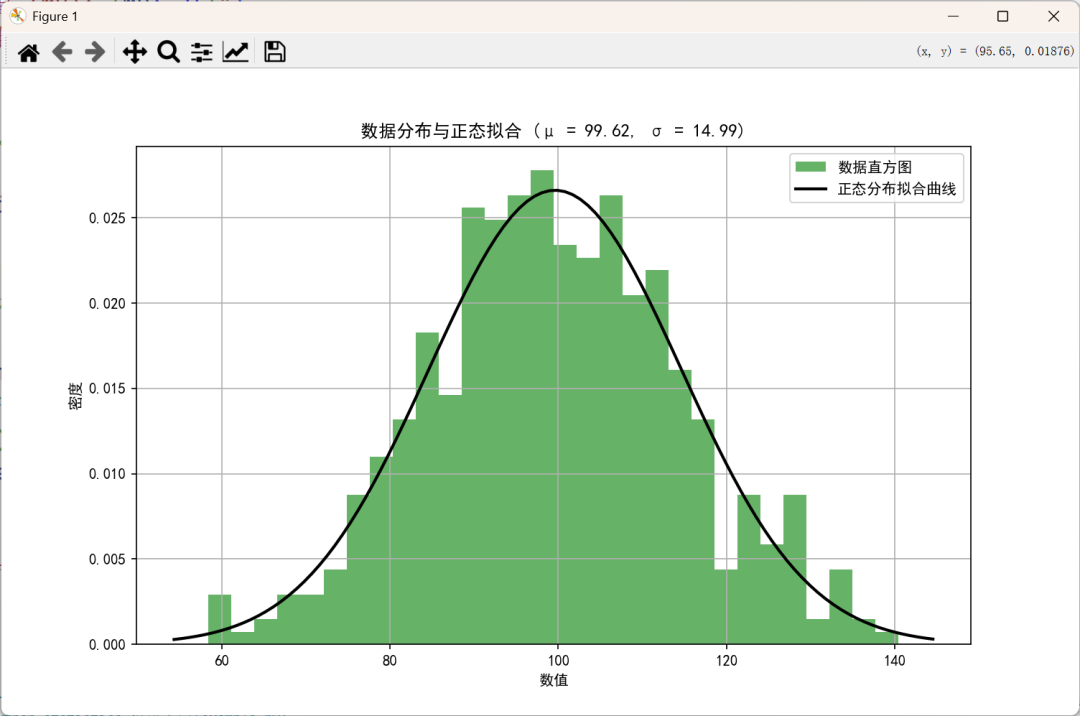
Analysis

• We first generated 500 random numbers with a mean of 100 and a standard deviation of 15 as sample data.
• <span>NormalDist.from_samples(sample_data)</span> learned from this data and created a normal distribution model.
• <span>plt.hist()</span> plotted the histogram of the original data. <span>density=True</span> is key here, ensuring that the vertical axis of the histogram represents “density” rather than “frequency”, making the total area equal to 1.
• We generated a smooth x-axis and used the model’s <span>.pdf()</span> method to calculate the theoretical normal curve.
• <span>plt.plot()</span> overlaid this curve on the histogram.

From the output chart, we can see that the outline of the green histogram bars matches the black normal curve quite well. This intuitively proves that our sample data can indeed be well described by a normal distribution.

Every day, we share Python programming knowledge, feel free to follow! If you find it helpful, please like and share!