Skyborn: Geostrophic Wind Calculation

Fundamentals of Geostrophic Wind Theory

Geostrophic wind is a core concept in atmospheric science, derived from the geostrophic balance assumption. When the horizontal pressure gradient force balances with the Coriolis force, the wind speed in the atmosphere is referred to as geostrophic wind. This theory is essential for understanding large-scale atmospheric circulation and has significant applications in weather forecasting, climate analysis, and atmospheric dynamics research.

Geostrophic Balance Equation

The mathematical expression for geostrophic balance is:

where is the Coriolis parameter, is the geostrophic wind vector, and is the geopotential height.

Expanded in component form:

Pain Points of Traditional Calculations

Calculating geostrophic wind using Python often faces the following issues:

Low computational efficiency: Python loops are time-consuming and slow
Complex implementation: Requires manual handling of spherical geometry, boundary conditions, coordinate transformations, and other details
Lack of standardization: Different implementation methods lead to consistency issues in results

Installation and Usage of Skyborn

System Requirements:

Python Version: 3.9 – 3.13
Operating System: Windows (x64), macOS (Intel/Apple Silicon), Linux (x86_64)

To install the Skyborn library, you can use pip:

pip install skyborn

Or use the following command:

pip install -U --index-url https://pypi.org/simple/ skyborn

Once installed, you can start using the geostrophic wind calculation features as described in this article.

Performance of Skyborn

Benchmark Testing

The performance test results of Skyborn are as follows:

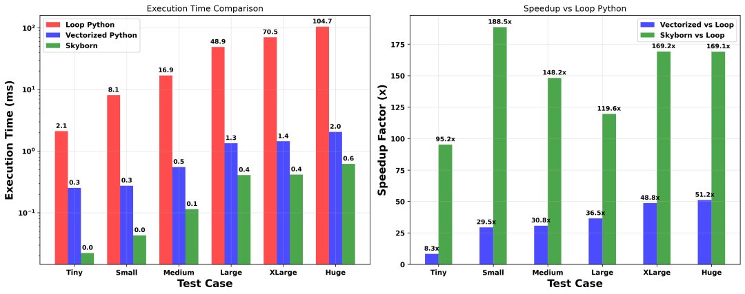
Skyborn: Geostrophic Wind Calculation — Performance Comparison Chart

Performance benchmark tests based on CESM data:

Test Scale	Range	Loop Python	Vectorized Python	Skyborn	Speedup Ratio
Tiny	60°N-40°N, 0°-60°E	2.1ms	0.3ms	0.03ms	95.2×
Small	70°N-30°N, 0°-120°E	8.1ms	0.3ms	0.04ms	188.5×
Medium	75°N-15°N, 0°-180°E	16.9ms	0.5ms	0.1ms	148.2×
Large	90°N-30°S, 0°-240°E	48.9ms	1.3ms	0.4ms	119.6×
XLarge	90°N-60°S, 0°-300°E	70.5ms	1.4ms	0.4ms	169.2×
Huge	Global	104.7ms	2.0ms	0.6ms	169.1×

Highlights of Performance Improvement:

Compared to traditional Python loops, Skyborn achieves a 95-189 times performance improvement
Even compared to optimized NumPy vectorized code, there is still a 30-51 times speedup
The computation time for global datasets has decreased from 104.7ms to 0.6ms, achieving high-speed calculations

Scientifically Rigorous Algorithms

The geostrophic wind calculation in Skyborn is strictly based on the fundamental equations of atmospheric dynamics, using finite difference methods in numerical analysis to solve the geostrophic balance equation. The algorithm implementation fully adheres to the following scientific principles:

Theoretical Foundation:

Based on quasi-geostrophic theory and geostrophic balance assumptions, it has good physical approximation in large-scale mid-latitude motion
Strictly follows the rules of vector operations in spherical coordinate systems, ensuring geometric accuracy in spatial gradient calculations
Uses standard geophysical parameters (gravitational acceleration g=9.80616 m/s², Earth radius Re=6371220 m, Earth’s rotation angular velocity Ω=7.292×10⁻⁵ rad/s), ensuring international consistency in calculation results

Numerical Methods:

Uses central difference format to calculate spatial derivatives, exhibiting second-order accuracy characteristics
Implements adaptive boundary condition handling, supporting periodic and non-periodic boundaries
Integrates a complete mechanism for detecting and handling missing values, ensuring data quality control

Practical Application Effects

The geostrophic wind calculation results for 500hPa geopotential height data in the mid-latitudes of the Northern Hemisphere are as follows:

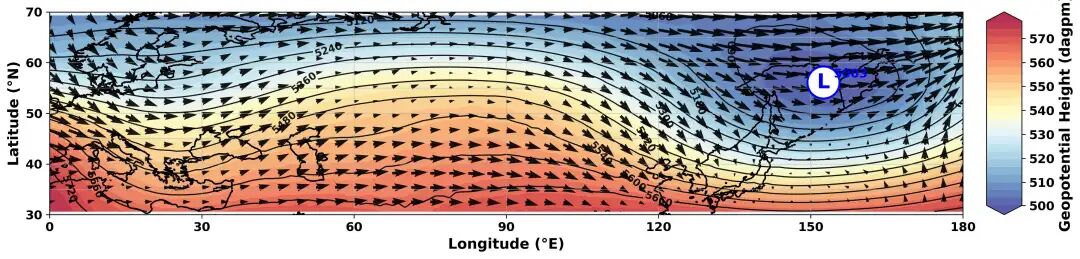
Based on geostrophic wind theory and the Coriolis effect, following the principle of “standing with the wind at your back, low on the left and high on the right”:

High-pressure center (anticyclone): In the Northern Hemisphere, it exhibits clockwise circulation. According to geostrophic wind theory, when standing with the wind at your back, the high-pressure system is on the right side, and the wind flows clockwise along the isohypses
Low-pressure center (cyclone): In the Northern Hemisphere, it exhibits counterclockwise circulation. When standing with the wind at your back, the low-pressure system is on the left side, and the wind flows counterclockwise along the isohypses

Plotting Code:

from skyborn.calc.geostrophic.xarray import geostrophic_wind
from skyborn.plot.plotting import add_equal_axes
import sys
import numpy as np
import xarray as xr
import matplotlib.pyplot as plt
import cartopy.crs as ccrs
import cartopy.feature as cfeature
from scipy import ndimage
sys.path.insert(0, "src/skyborn")

def plot_circulation():
    filepath = "z_data.nc"
    ds = xr.open_dataset(filepath)
    z = ds.z / 9.8

    z_region = z.sel(time='2019-01', level=500.0,
                      lat=slice(70, 30), lon=slice(0, 180)).squeeze()

    # Use xarray interface to calculate geostrophic wind
    wind_result = geostrophic_wind(z_region, missing_value=-999.0)
    ug = wind_result.ug.values
    vg = wind_result.vg.values

    z_data = z_region.values
    glat = z_region.lat.values
    glon = z_region.lon.values

    z_smooth = ndimage.gaussian_filter(z_data, sigma=1.5)

    local_maxima = ndimage.maximum_filter(z_smooth, size=10) == z_smooth
    local_minima = ndimage.minimum_filter(z_smooth, size=10) == z_smooth

    local_maxima[0:3, :] = local_maxima[-3:,
                                        :] = local_maxima[:, 0:3] = local_maxima[:, -3:] = False
    local_minima[0:3, :] = local_minima[-3:,
                                        :] = local_minima[:, 0:3] = local_minima[:, -3:] = False

    max_coords = np.where(local_maxima)
    min_coords = np.where(local_minima)

    max_values = z_smooth[max_coords]
    min_values = z_smooth[min_coords]

    z_std = np.std(z_smooth)
    z_mean = np.mean(z_smooth)

    significant_maxima = max_values > (z_mean + 1.0 * z_std)
    significant_minima = min_values < (z_mean - 1.0 * z_std)

    max_coords = (max_coords[0][significant_maxima],
                  max_coords[1][significant_maxima])
    min_coords = (min_coords[0][significant_minima],
                  min_coords[1][significant_minima])

    fig, ax = plt.subplots(1, 1, figsize=(16, 10), subplot_kw={
                           'projection': ccrs.PlateCarree()})

    lon_grid, lat_grid = np.meshgrid(glon, glat)

    z_levels = np.linspace(z_data.min(), z_data.max(), 25)
    contourf = ax.contourf(lon_grid, lat_grid, z_data, levels=z_levels,
                           cmap='RdYlBu_r', transform=ccrs.PlateCarree(), alpha=0.8,
                           extend='both')

    contour_levels = np.arange(5000, 5800, 60)
    contour = ax.contour(lon_grid, lat_grid, z_data, levels=contour_levels,
                         colors='black', linewidths=1.2, alpha=0.9,
                         transform=ccrs.PlateCarree())
    clabels = ax.clabel(contour, inline=True, fontsize=10, fmt='%d')
    for txt in clabels:
        txt.set_fontweight('bold')

    skip = 3
    ax.quiver(lon_grid[::skip, ::skip], lat_grid[::skip, ::skip],
              ug[::skip, ::skip], vg[::skip, ::skip],
              scale=1000, scale_units='width', alpha=0.9,
              transform=ccrs.PlateCarree(), color='black',
              width=0.003)

    for i in range(len(max_coords[0])):
        lat_idx, lon_idx = max_coords[0][i], max_coords[1][i]
        lat_pos, lon_pos = glat[lat_idx], glon[lon_idx]
        value = z_data[lat_idx, lon_idx]
        ax.text(lon_pos, lat_pos, 'H', color='red', fontsize=20, fontweight='bold',
                transform=ccrs.PlateCarree(), ha='center', va='center',
                bbox=dict(boxstyle="circle,pad=0.3", facecolor='white', edgecolor='red', linewidth=2))
        ax.text(lon_pos+2, lat_pos+1, f'{int(value)}', color='red', fontsize=12, fontweight='bold',
                transform=ccrs.PlateCarree())

    for i in range(len(min_coords[0])):
        lat_idx, lon_idx = min_coords[0][i], min_coords[1][i]
        lat_pos, lon_pos = glat[lat_idx], glon[lon_idx]
        value = z_data[lat_idx, lon_idx]
        ax.text(lon_pos, lat_pos, 'L', color='blue', fontsize=20, fontweight='bold',
                transform=ccrs.PlateCarree(), ha='center', va='center',
                bbox=dict(boxstyle="circle,pad=0.3", facecolor='white', edgecolor='blue', linewidth=2))
        ax.text(lon_pos+2, lat_pos+1, f'{int(value)}', color='blue', fontsize=12, fontweight='bold',
                transform=ccrs.PlateCarree())

    ax.add_feature(cfeature.COASTLINE, linewidth=1.5)
    ax.add_feature(cfeature.LAND, alpha=0.3, color='lightgray')
    ax.add_feature(cfeature.OCEAN, alpha=0.3, color='lightblue')

    ax.set_xlim(0, 180)
    ax.set_ylim(30, 70)
    ax.gridlines(draw_labels=False, alpha=0.5)

    ax.set_xticks(np.arange(0, 181, 30))
    ax.tick_params(axis='x', which='major', labelsize=12,
                   top=False, labeltop=False, bottom=True, labelbottom=True)

    ax.set_yticks(np.arange(30, 71, 10))
    ax.tick_params(axis='y', which='major', labelsize=12,
                   left=True, labelleft=True, right=False, labelright=False)

    for label in ax.get_xticklabels():
        label.set_fontweight('bold')
    for label in ax.get_yticklabels():
        label.set_fontweight('bold')

    ax.set_xlabel('Longitude (°E)', fontsize=14, fontweight='bold')
    ax.set_ylabel('Latitude (°N)', fontsize=14, fontweight='bold')

    cax = add_equal_axes(ax, 'right', 0.02, 0.03)
    cbar = plt.colorbar(contourf, cax=cax, orientation='vertical')
    cbar.set_label('Geopotential Height (dagpm)',
                   fontsize=14, fontweight='bold')

    cbar_ticks = np.arange(500, 580, 10)
    cbar.set_ticks(cbar_ticks * 10)
    cbar.set_ticklabels([f'{int(tick)}'for tick in cbar_ticks])
    cbar.ax.tick_params(labelsize=12)
    for label in cbar.ax.get_yticklabels():
        label.set_fontweight('bold')

    plt.show()


if __name__ == "__main__":
    plot_circulation()

Flexible API Design

Skyborn provides three usage methods to meet different user needs:

1. NumPy Interface – Low-level Array Calculations

import numpy as np
import xarray as xr
from skyborn.calc.geostrophic import geostrophic_wind

# Load ERA5 geopotential height data
ds = xr.open_dataset('era5_zdata.nc')
z_region = ds.z.sel(level=500) / 9.80665# Select 500hPa layer, convert to geopotential height (gpm)

# Extract numpy array and coordinates
z_data = z_region.values  # Geopotential height data (nlat, nlon)
glat = z_region.lat.values  # Latitude array
glon = z_region.lon.values  # Longitude array

# Directly calculate geostrophic wind
ug, vg = geostrophic_wind(z_data, glon, glat, 'yx', missing_value=-999.0)

2. xarray Function Interface – Fast Calculation

import xarray as xr
from skyborn.calc.geostrophic.xarray import geostrophic_wind

# Load ERA5 geopotential height data
ds = xr.open_dataset('era5_zdata.nc')
z_region = ds.z.sel(level=500) / 9.80665  # Select 500hPa layer, convert to geopotential height (gpm)

# xarray interface: automatic coordinate detection, one-liner calculation
wind_result = geostrophic_wind(z_region, missing_value=-999.0)
ug = wind_result.ug.values  # Zonal wind component
vg = wind_result.vg.values  # Meridional wind component

3. xarray Class Interface – Object-Oriented Analysis

import xarray as xr
from skyborn.calc.geostrophic.xarray import GeostrophicWind

# Load ERA5 geopotential height data
ds = xr.open_dataset('era5_zdata.nc')
z_data = ds.z.sel(level=500) / 9.80665# Select 500hPa layer, convert to geopotential height (gpm)

# Create geostrophic wind analysis object
gw = GeostrophicWind(z_data, missing_value=-999.0)

# Get wind components
ug, vg = gw.uv_components()

# Calculate geostrophic wind speed
wind_speed = gw.speed()

# Access original data
original_z = gw.geopotential_height
lon_coords = gw.longitude
lat_coords = gw.latitude

Recommendation: For most users, it is recommended to use the xarray function interface for simplicity.

Summary

Outstanding Performance: Skyborn employs efficient algorithm optimizations for ultra-fast calculations
Easy to Use: Supports NumPy and xarray interfaces with automatic coordinate detection
Comprehensive Functionality: Supports 2D/3D/4D multidimensional data processing
Stable and Reliable: Complete boundary handling and outlier detection

Application Scenarios

Educational Applications

Atmospheric Science Education: Provides students with intuitive demonstrations of geostrophic wind calculations, validating the integration of theory and practice
Experimental Courses: Supports multidimensional data processing, suitable for undergraduate and graduate course experiments
Learning Threshold: Simple API design lowers the learning threshold, allowing students to focus on the scientific issues themselves

Production Applications

Numerical Weather Prediction Systems: Efficient computational performance meets the real-time requirements of operational forecasting
Climate Analysis Operations: Supports large-scale historical data processing, suitable for climate monitoring and analysis
Wind Field Diagnosis and Visualization: Provides accurate wind field analysis products for meteorological services
Real-time Weather Analysis Systems: High-speed computational performance supports frequent real-time analysis needs

Research Applications

Atmospheric Dynamics Analysis: Accurate geostrophic wind calculations support the study of complex dynamical mechanisms
Climate Model Validation: Provides high-precision diagnostic analysis tools for model outputs
Meteorological Data Processing: Integrated into automated processing systems to improve research efficiency

Conclusion

The Skyborn geostrophic wind calculation module provides an efficient and accurate numerical computing solution for the atmospheric science community.

Get Skyborn:

pip install skyborn

❝

For more information, please refer to the Skyborn documentation —————https://skyborn.readthedocs.io/en/latest/

Reference

[1] Holton, J. R., & Hakim, G. J. (2012). An introduction to dynamic meteorology (5th ed.). Academic Press.

[2] Vallis, G. K. (2017). Atmospheric and oceanic fluid dynamics: Fundamentals and large-scale circulation (2nd ed.). Cambridge University Press.

[3] Peixoto, J. P., & Oort, A. H. (1992). Physics of climate. American Institute of Physics.

[4] Washington, W. M., & Parkinson, C. L. (2005). An introduction to three-dimensional climate modeling (2nd ed.). University Science Books.

[5] Kalnay, E. (2003). Atmospheric modeling, data assimilation and predictability. Cambridge University Press.

[6] Trenberth, K. E. (1991). Climate diagnostics from global analyses: Conservation of mass in ECMWF analyses. Journal of Climate, 4(7), 707-722.