Table of Contents
1. Introduction to Robotic Arm Algorithms
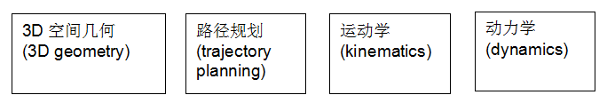
2. Kinematics Section2.1.1. Rigid Body Tree2.1.2. Inverse Kinematics Algorithm2.1.3. Simulink Example

1Introduction to Robotic Arm Algorithms
MATLAB launched the Robotics System Toolbox (RST) in 2016, which includes many algorithms related to robotic arms. With the increasing demand from customers, new features are also being added. To help readers understand more about the support RST provides for robotic arms, let’s take a look at an overview of the algorithms related to robotic arms.
These terms may sound complex, but they are very useful in the world of robotic arms. Let’s look at a simple example. The following diagram shows a simple schematic of a robotic arm: the end-effector of the robotic arm is influenced by four rotational joints and three links, allowing it to reach different working locations and to be in different rotational angles.
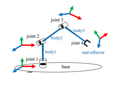
To analyze the specific position and angle of the end-effector, we see that it performs four rotations and three translations relative to the base. The total of these four rotations and three translations can be represented by a matrix:
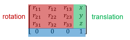
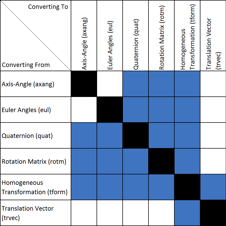
This matrix is also called a Homogeneous Transformation. Sometimes, there are different representations for rotation, such as Euler Angles, Quaternions, Rotation Matrices, etc.; for translation, a Translation Vector can also be used. With RST, all of these can be easily interchanged through different functions. The following diagram shows a specific list of functions:
 For example:
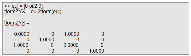
Convert Euler Angles to Homogeneous Transformation.
Since the lengths of the robotic arm’s links are known, once the angles of each joint’s rotation are determined, we can ascertain the final position and orientation of the end-effector.This is referred to as forward kinematics. Conversely, if we know the final position and orientation of the end-effector, we can deduce the angles of each joint, which is known as inverse kinematics. The primary focus of robotic arms is on inverse kinematics.
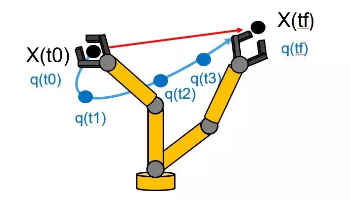
If the end-effector needs to traverse a relatively long path from point A to point B, we need to plan a series of waypoints to ensure a smooth path for the end-effector, which is referred to as trajectory planning or motion interpolation.
For example, in the diagram below:The blue curve is called the path, while the various waypoints along the path are called the trajectory. A clear indicator of how to design the trajectory passing through these waypoints is “smoothness”. What does “smooth” mean? It could imply “continuous speed”, “continuous acceleration”, “no jerks”, etc. These indicators will be translated into mathematical algorithms. RST also provides corresponding algorithm support, and the author will write another article describing this after the release of MATLAB 2019a.
The joint positions of the robotic arm are generally driven by motors.The motors generate torque to rotate the mechanical devices, driving the robotic arm. The required torque varies depending on the situation or timing.
For example:
- When the robotic arm is placed horizontally, the joint motors need to generate torque to counteract the force of gravity;
- When the robotic arm needs to move quickly, the required torque is greater than when moving slowly. When the robotic arm bends or extends, the center of gravity changes, and due to the difference in inertia (I = mr²), the required joint torque also varies;
-
Additionally, in many situations, the robotic arm needs to interact with humans (collaborative robots), and when it encounters a human body, it needs to perform safe protective actions and adjust the torque accordingly.
These factors that need to consider torque are referred to as dynamics. Similar to kinematics, dynamics is divided into forward dynamics and inverse dynamics. RST supports both with corresponding MATLAB functions and Simulink blocks. The author will also write another article detailing the dynamics section of RST.
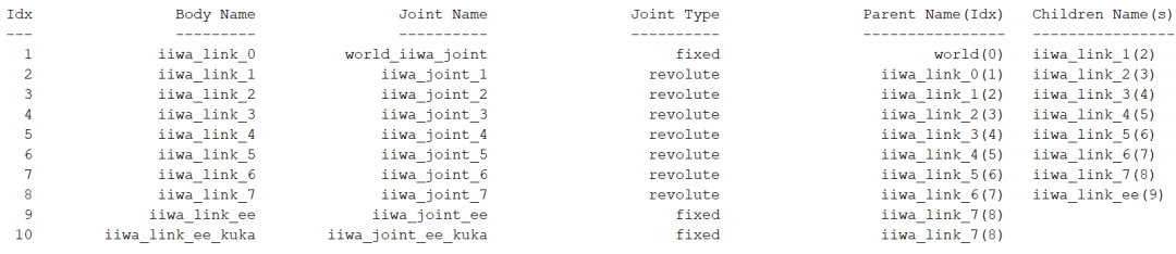
2Kinematics Section2.1.1Rigid Body Tree
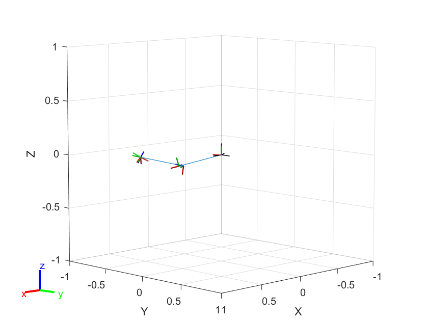
When we study kinematics (mainly inverse kinematics), we are examining how the change in the position of the end-effector affects the angles of each joint. RST uses an object called Rigid Body Tree, which makes kinematic design user-friendly and visual. The diagram below shows an example of a robotic arm’s rigid body tree, displaying the detailed parameters of each body in the MATLAB interface.
Generally, the Rigid Body Tree is directly imported from the CAD file of the robotic arm or a URDF (Unified Robot Description Format) file. However, it also supports step-by-step addition of each body.
Let’s type a few MATLAB commands:
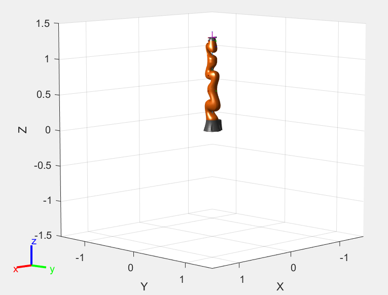
robot = importrobot(‘iiwa14.urdf’);
show(robot);
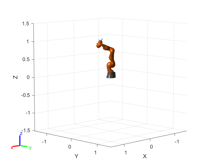
Let’s change the angles of the robot’s joints (configuration), for example, let MATLAB automatically provide a random angle configuration and see the result. Clearly, the angles have changed.
q=randomConfiguration(robot);
show(robot,q);
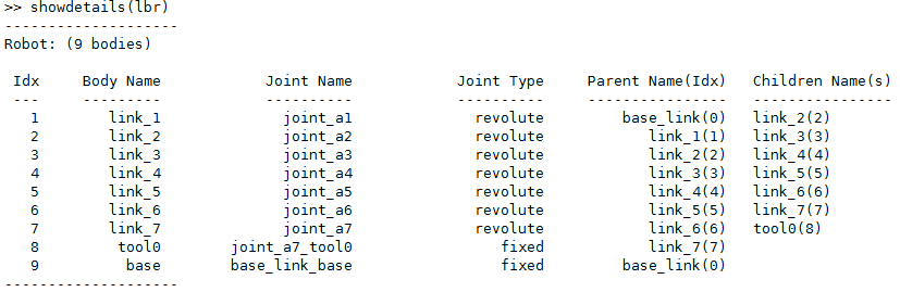
What is the end-effector of this robotic arm?
showdetails(robot)
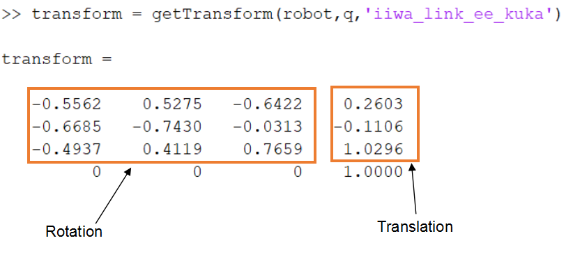
Let’s also look at the Homogeneous Transformation of the end-effector relative to the robot’s base (relative position and angle).
2.1.2Inverse Kinematics Algorithm
The inverse kinematics algorithm can be solved in two ways: one is analytical solutions; the other is numerical solutions. MATLAB uses numerical solutions, which can be understood as iterative optimization or approximate solutions.
There are two inverse kinematics solvers in MATLAB:1. Inverse Kinematics2. Generalized Inverse Kinematics
The difference between the two is that the latter has many more constraints than the former. For example, constraints on the direction of the end-effector, angle constraints for each joint of the robotic arm, position constraints, etc.
Let’s first look at the simpler Inverse Kinematics
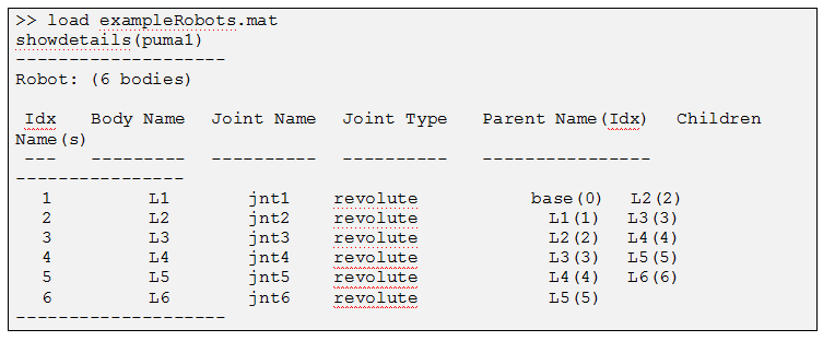
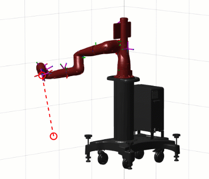
This is a 6-axis robot, and the end-effector is L6.
randConfig = puma1.randomConfiguration;
tform = getTransform(puma1,randConfig,’L6′,’base’);
show(puma1,randConfig);
The desired final result is shown in the following image:
tform is the position and orientation of L6 relative to the base (collectively referred to as pose).
The following MATLAB code calculates the angles of each joint (configSoln) at the end, using an iterative numerical solution, where weights are the weights and initialguess is an initial estimate.
ik = robotics.InverseKinematics(‘RigidBodyTree’,puma1);
weights = [0.25 0.25 0.25 1 1 1];
initialguess = puma1.homeConfiguration;
[configSoln,solnInfo] = ik(‘L6’,tform,weights,initialguess);
Now let’s look at the more complex Generalized Inverse Kinematics:
The following code does several things:
a) Imports a 7-degree-of-freedom robotic arm — sawyer
b) Sets the constraints for the inverse kinematics solver – for example, the end-effector of the robotic arm always points to an object on the ground
c) Solves the inverse kinematics
sawyer = importrobot(‘sawyer.urdf’, ‘MeshPath’, …
fullfile(fileparts(which(‘sawyer.urdf’)),’..’,’meshes’,’sawyer_pv’));
gik = robotics.GeneralizedInverseKinematics(‘RigidBodyTree’,sawyer, …
‘ConstraintInputs’,{‘position’,’aiming’});
% Target Position constraint
targetPos = [0.5, 0.5, 0];
handPosTgt = robotics.PositionTarget(‘right_hand’,’TargetPosition’,targetPos);
% Target Aiming constraint
targetPoint = [1, 0, -0.5];
handAimTgt = robotics.AimingConstraint(‘right_hand’,’TargetPoint’,targetPoint);
% Solve Generalized IK
[gikSoln,solnInfo] = gik(sawyer.homeConfiguration,handPosTgt,handAimTgt)
show(sawyer,gikSoln);
If we add a segment that changes the position of the end-effector and call this code for the animation effect, you will find that the direction of the end-effector does not change – the constrained inverse dynamics solution was successful:
2.1.3Simulink ExampleAfter installing RST, several blocks related to robotic arms will appear in the Simulink library:Among them, Inverse Kinematics is the inverse kinematics block, while other modules are related to dynamics, which I will focus on in the next article.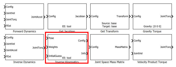
Search for “Designing Robot Manipulator Algorithms” on MATLAB Central File Exchange, which is an example based on Simulink and Stateflow. Let’s first look at the running results:
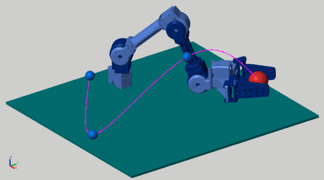
This example demonstrates the robotic arm’s end-effector grabbing a red object, moving along the planned purple trajectory. The stateflow state machine below is a trajectory tracking algorithm, which ensures that the end-effector moves along the preset trajectory.
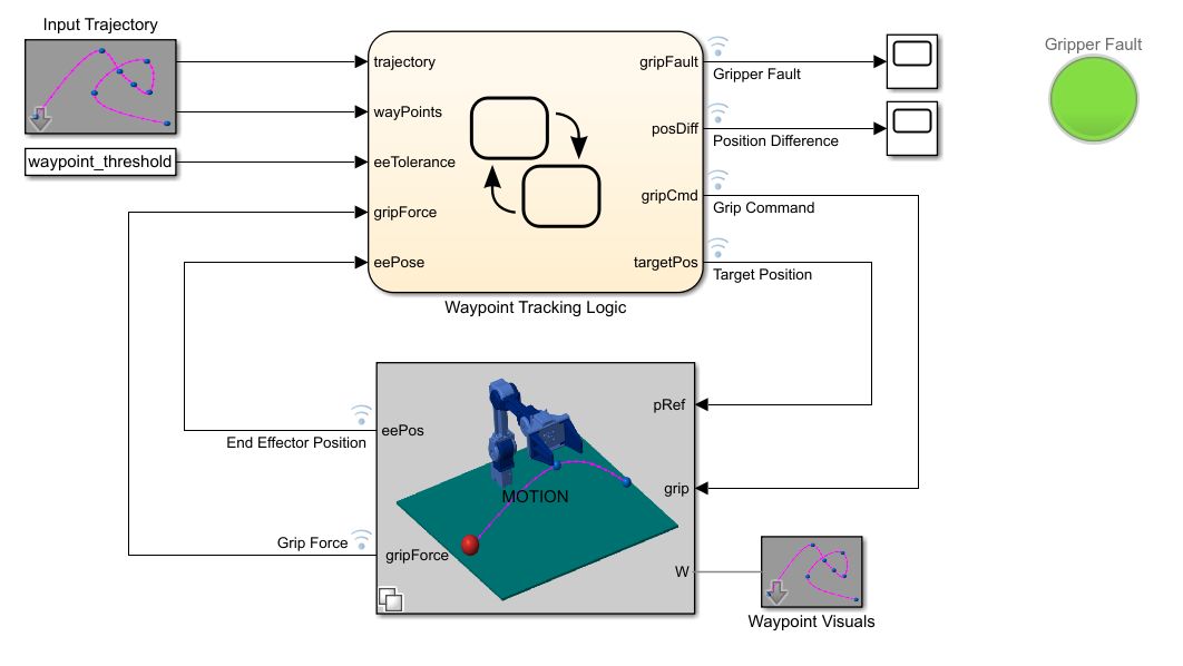
The state machine below is the motion control part and the environment and physical model. The motion control is straightforward – it directly calculates the inverse kinematics and sends the calculated joint angles to the physical model for display. The physical model construction is also simple – just import the robotic arm’s URDF file using SimScape’s SimMultibody.
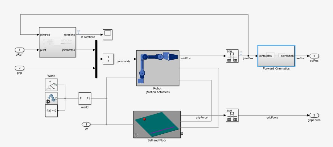 Here, we can see that the physical model does not include servo motors, but rather “transparent transmission” – the results of the inverse kinematics are directly sent to the mechanical model for display. In reality, the motion controller would send position, speed, and torque commands through a servo bus (such as EtherCAT) to each joint’s motor for execution, with the motors driving the mechanical structure through reducers.For example,
A 6-axis robotic arm will have 6 servo motors, and the motion controller will parse the motion process into position, speed, and torque commands that the 6 motors can understand.If you want to gain a deeper understanding of the mechanical model + motor model + motor control + motion control, you can search for “How a Differential Equation Becomes a Robot” on the MathWorks website. This is a series of videos that will sequentially explain the above technical points.
Follow MathWorks’ subscription account
Learn more about MATLAB robotic arm algorithms