For comparative studies on hyperparameter optimization methods, refer to the following articles:
Hyperparameter Tuning Based on Bayesian Optimization-1
Jethro, WeChat Official Account: Xiaobailou Laboratory 【MATLAB Reinforcement Learning Toolbox】 Hyperparameter Tuning Based on Bayesian Optimization-1
01
—
Bayesian Optimization Algorithm
Basic Principle:
The Bayesian optimization algorithm is a global optimization method used to minimize a scalar objective function f(h) within a bounded domain (where h represents the set of hyperparameters to be optimized). This objective function can be deterministic or stochastic, meaning that it may return different results when evaluated at the same input variable h. Furthermore, the components of the input variable h can be continuous real numbers, integers, or categorical variables, i.e., a discrete set of names [1]. The core idea of Bayesian optimization is to predict the behavior of the objective function at unassessed points by constructing a probabilistic model (such as a Gaussian process model) and selecting the optimal sampling point for evaluation based on these predictions. This process typically includes the following steps, as illustrated in Figure 1 [2,3]:
Initialization: Start sampling from random points and evaluate the objective function values.
Update Model: Update the probability distribution of the objective function using a Gaussian process or other statistical models based on existing observational data.
Select Next Sampling Point: Decide the next point to evaluate through a strategy called the “Acquisition Function.” Common acquisition functions include Expected Improvement, Probability of Improvement, and Lower Confidence Bound.
Iterative Optimization: Repeat the above steps until a stopping criterion is met (such as reaching the maximum number of iterations or finding a sufficiently good solution).
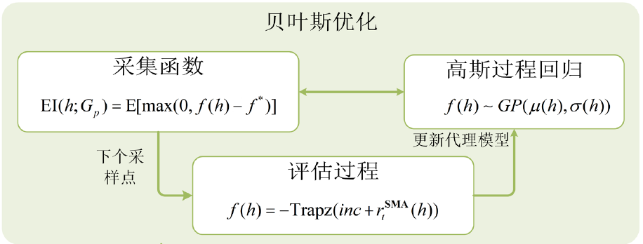
Figure 1 Structure Diagram of Bayesian Optimization
Note: h represents the set of hyperparameters; Gp represents the posterior distribution of the Gaussian regression process; f* represents the currently obtained best Gaussian process regression function value; μ(h) and σ(h) represent the mean and variance of the objective function f(h) under the selected candidate hyperparameter set h; Trapz() represents a custom objective function; for specific meanings, please refer to the literature.
Objective Function:
The bayesopt command attempts to minimize the objective function (objective function). Specifically, when a function needs to be maximized, simply set the objective function to the negative value of the function to be maximized. For example, if the objective function is f(h), then -f(h) should be set as the objective function for bayesopt. In this way, bayesopt will attempt to minimize -f(h), thereby achieving the effect of maximizing f(h). Bayesopt will pass a variable table to the objective function, these variables having the declared names and types. Additionally, the objective function can return extra information, such as coupled constraints and user data, which help with constraint handling and result analysis during the optimization process.
The syntax of the objective function is as follows:
[objective,coupledconstraints,userdata] = fun(h)%objective — The value of the objective function at point h, a real number;%coupledconstraints - The value of coupled constraints (if any, optional output), a real value vector. %Negative values indicate that constraints are met, positive values indicate unmet constraints.%userdata — The function can return optional data for further use, such as for plotting or logging (optional output).Variable Settings:
In MATLAB, use the optimizableVariable function to create variable description objects for Bayesian optimization. Each variable has a unique name and value range. The basic syntax for creating a variable is as follows:
variable = optimizableVariable(Name,Range)%where Name is the variable name, Range is the variable value range,%For continuous and integer variables, Range is a vector containing the lower and upper bounds;%For categorical variables, Range is a cell array containing possible value names.Variable Types: The Type parameter specifies the following three types:
‘real’: Continuous real values between finite bounds. The vector [lower upper] is the variable range Range, indicating lower and upper bounds.
‘integer’: Integer values within a finite range, similar to ‘real’.
‘categorical’: A cell array of possible value names specified in the Range parameter, such as {‘red’,’green’,’blue’}.
Log Transformation: For ‘real’ and ‘integer’ type variables, the bayesopt can specify searching in the logarithmic scale space by setting the Transform name-value pair to ‘log’. For this transformation, ensure that the lower bound of Range is strictly positive (for ‘real’ type) or non-negative (for ‘integer’ type). For example:
var2 = optimizableVariable('ivar',[1 1000],'Type','integer','Transform','log')Bayesopt’s range includes endpoints. Therefore, 0 cannot be used as the lower limit for logarithmic transformation variables. If you want to set the lower limit of ivar to 0 in a logarithmic transformation variable, you can set the lower limit of ivar to 1 and then use ivar-1 in the objective function. Log transformation can convert the multiplicative operations of the original data into additive operations, making numerical calculations more stable and avoiding underflow or overflow issues caused by excessively large numbers. In Bayesian optimization, log transformation can compress the value range of the objective function into a smaller range, thus reducing the sparsity problem of the data.
Excluding Variables: If you want to exclude a certain parameter (e.g., ivar) from the optimization, you can handle it by setting ivar.optimize=false.
Acquisition Function Types:
In Bayesian optimization, the acquisition function is one of the key components, mainly responsible for determining the location of the next sampling point. It quantifies the value of each potential sampling point by combining the predicted values of the surrogate model and uncertainties, thus guiding the next choice in the optimization process. Specifically, the acquisition function needs to strike a balance between exploration and exploitation to avoid getting stuck in local optima and to quickly find the global optimum. Here are six common types of acquisition functions and their characteristics:
Expected Improvement (EI):
'expected-improvement'EI is one of the most popular acquisition functions, performing excellently in balancing exploration and exploitation. EI calculates the potential improvement that candidate points may bring compared to the current optimal value, considering uncertainty. EI is suitable for most situations, but its downside is that it may get stuck in local optima in certain cases.
Expected Improvement Plus (EI+):
'expected-improvement-plus'EI+ adds extra parameters on top of EI to reduce the risk of getting stuck in local optima. It starts with a larger parameter value during the initial sampling and gradually decreases as the number of samples increases, thus tending to explore more in the early stages.
Expected Improvement Per Second (EI/s):
'expected-improvement-per-second'EI/s is designed for situations with limited computational resources, optimizing the efficiency of each iteration by considering time costs.
Expected Improvement Per Second Plus (EI/s+):
'expected-improvement-per-second-plus' (default)EI/s+ is the default acquisition function selected by MATLAB, combining the advantages of EI/s and EI+, considering both time costs and avoiding the issue of getting stuck in local optima.
Lower Confidence Bound (LCB):
'lower-confidence-bound'LCB is an acquisition function that tends to explore, selecting the next sampling point based on confidence intervals. LCB is suitable for situations requiring extensive exploration, as it tends to sample points with higher uncertainty.
Probability of Improvement (PI):
'probability-of-improvement'PI calculates the probability that candidate points can improve the current optimal value. PI leans more towards exploitation, as it only considers whether it can improve the current optimal value, not the magnitude of the improvement.
Acquisition Function Selection Experience:
-
If you want to explore unknown areas more in the early stages, you can choose LCB or PI.
-
If you want to balance exploitation and exploration, EI is a good choice.
-
If computational resources are limited and you want to improve efficiency, you can choose EI/s or EI/s+.
-
If you are concerned about getting stuck in local optima, you can choose EI+ or EI/s+.
Therefore, when selecting an acquisition function, you should decide the most suitable type based on optimization goals, computational resources, and preferences for exploration versus exploitation.
02
—
Examples of Bayesian Optimization Applications
Utilizing the official MATLAB example “Tune Hyperparameters Using Bayesian Optimization” [4] to study the application of Bayesian optimization algorithms in hyperparameter optimization for deep reinforcement learning. In this example, we use the bayesopt (Statistics and Machine Learning Toolbox) [5] command to optimize hyperparameters.
Create Environment:
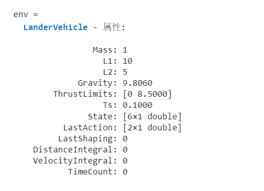
The landing vehicle environment used in this example is the same as the official example “Train PPO Agent for a Lander Vehicle” [6]
View environment code and open the environment:
open("LanderVehicle.m"); % Note to navigate to the file directory first env = LanderVehicle();% Create environmentThe environment characteristics are shown as output:
When optimizing hyperparameters for the Proximal Policy Optimization (PPO) algorithm, the hyperparameters to be optimized and their ranges can be specified using the ‘optimizableVariable’ function.
Detailed descriptions of hyperparameters and their setting ranges:
Experience Horizon
-
Range: 100 ~ 1000
-
Description: The larger the experience horizon, the better the stability of training. A larger experience horizon can more comprehensively capture changes in the environment, thus improving learning effectiveness.
Mini-batch Size
-
Range: 50 ~ 100
-
Description: A smaller mini-batch size calculates efficiently but may introduce larger variance; a larger size improves training stability but requires more memory.
Learning Rates of Actor and Critic Networks
-
Range: 1e-6 ~ 1e-2
-
Description: A learning rate that is too high can lead to drastic updates, potentially causing chaotic action selection, so it needs to be set cautiously.
Discount Factor
-
Range: 0.95 ~ 1.0
-
Description: Controls the importance of long-term rewards; the closer the discount factor is to 1, the greater the influence of future rewards.
Number of Epochs
-
Range: 1 ~ 10
-
Description: Specifies the number of learning epochs conducted in each update, which can affect the convergence speed and stability of training.
Clipping Factor
-
Range: 0.01 ~ 0.1
-
Description: Used to limit changes in each policy update step, ensuring that the policy updates are not too aggressive, thus improving training stability.
Entropy Coefficient
-
Range: 0.01 ~ 0.1
-
Description: The larger the value, the stronger the agent’s exploration ability, helping to avoid premature convergence to local optima.
% Mini-batch size (Mini-batch size) mbsz = optimizableVariable( ... 'MiniBatchSize', ... % Name [50,500], ... % Range 'Type','integer'); Type % experience horizon hrz = optimizableVariable( ... 'ExperienceHorizon', ... [100 600], ... 'Type','integer'); % actor and critic learning rates actor lr = optimizableVariable('ActorLearnRate',[1e-6,1e-2]); critic lr = optimizableVariable('CriticLearnRate',[1e-6,1e-2]); % clip factor clip f = optimizableVariable('ClipFactor',[0.01,0.1]); % entropy loss weight ent w = optimizableVariable('EntropyLossWeight',[0.01,0.1]); % number of epochs nepoch = optimizableVariable('NumEpoch',[1,10],'Type','integer'); % discount factor disc f = optimizableVariable('DiscountFactor',[0.95,1.0]);<span>Creating the vector of hyperparameters to be optimized</span>
optimVars = [mbsz,hrz,actorlr,criticlr,clipf,entw,nepoch,discf];Defining the Objective Function:
The objective function trains a PPO agent using a set of hyperparameters and returns a score representing the optimality of the hyperparameters. The cumulative return gained by the PPO agent during a single training session can be specified as the objective function value. Minimizing this score can enhance the agent’s performance.
The function performs the following steps:
-
(1) Create the agent object using a network with 400 units in the hidden layer.
-
(2) Configure the agent’s hyperparameters using the input params. params is a structure containing the hyperparameters configured in the previous section.
-
(3) Train the agent for 3000 episodes, with a maximum of 600 steps per episode.
-
(4) Evaluate the agent every 20 trainings, conducting 5 simulations for each evaluation.
Returns the objective (the score from the last evaluation), constraints, and user data (the trained agent and training results) as function outputs.
function [objective,constraints,UserData] = objectiveFun(params,env) % Fix random seed for reproducibility rng(0,"threefry"); % Get state and action information from the environment obsInfo = getObservationInfo(env); actInfo = getActionInfo(env); % Set PPO agent network options % Set Hidden unit specifications initOpts = rlAgentInitializationOptions(NumHiddenUnit=400); % NumHiddenUnit - The number of units in each hidden fully connected layer of the DRL agent's network (excluding the fully connected layer before network output), specified as a positive integer. % This value also applies to any LSTM layers. % Set PPO agent options and configure hyperparameters % Input variables take params % rlOptimizerOption sets optimization options for Actor and Critic actorOpts = rlOptimizerOptions( ... LearnRate=params.ActorLearnRate, ... GradientThreshold=1); criticOpts = rlOptimizerOptions( ... LearnRate=params.CriticLearnRate, ... GradientThreshold=1); % GradientThreshold specifies the gradient threshold for training the Actor or Critic function approximator, specified as Inf or a positive scalar. % If the gradient exceeds this value, gradient clipping will be performed according to the specified gradient threshold method. % Gradient clipping limits the change in network parameters during training iterations. agentOpts = rlPPOAgentOptions(... ExperienceHorizon = params.ExperienceHorizon,... ClipFactor = params.ClipFactor,... EntropyLossWeight = params.EntropyLossWeight,... ActorOptimizerOptions = actorOpts,... CriticOptimizerOptions = criticOpts,... MiniBatchSize = params.MiniBatchSize,... NumEpoch = params.NumEpoch,... SampleTime = 0.1,... DiscountFactor = params.DiscountFactor); % Create PPO agent agent = rlPPOAgent(obsInfo,actInfo,initOpts,agentOpts); % Training options % The agent trains for a maximum of 3000 episodes, with a maximum of 600 steps per episode % Do not store training data during training, do not display training curves training-plot trainOpts = rlTrainingOptions(... MaxEpisodes = 3000,... % Training episodes MaxStepsPerEpisode = 600,... % Steps per episode StopTrainingCriteria = "none",... % Do not set stop training criteria SimulationStorageType = "none",... % Do not store data b Plots = "none",... % Do not display training process curves b Verbose = false); % Do not display training process in command line % Agent evaluation evl = rlEvaluator(EvaluationFrequency=20, NumEpisodes=5); % Training result = train(agent, env, trainOpts, Evaluator=evl); % Objective function score score = result.EvaluationStatistic; score(isnan(score)) = []; objective = -score(end); % Constraint settings, no constraints in this example constraints = []; % Store the training results and mature agent in user data UserData.TrainingResult = result; UserData.Agent = agent; endBayesian Optimization:
Fix the random data stream for reproducibility. The output previousRngState is a structure containing information about the previous state of the stream.
previousRngState = rng(0,"twister")Create an anonymous function handle for the objective function. This allows the environment object env to be passed to the objective function.
objFun = @(params) objectiveFun(params,env);Optimize hyperparameters using the bayesopt command
-
Pass objFun and optimVars as input parameters.
-
Run optimization using parallel workers. This requires the Parallel Computing Toolbox™ software. If this software is not installed, set UseParallel to false.
-
Due to the high computational load of the optimization process, it may take several hours to complete, so load previously adjusted results. If you want to run the optimization algorithm, set runOptimization to true.
runOptimization = false; % true/false if runOptimization % Train using Bayesian optimization optimResults = bayesopt(objFun,optimVars,UseParallel=true); else % Load previously run results load("LanderOptimResults.mat","optimResults"); end03
—
Result Analysis
Plot a comparison chart of the minimum observed values and estimated values against the number of function evaluations.
plot(optimResults,@plotMinObjective)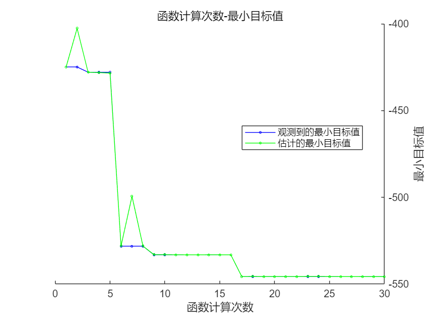
Bayesian optimization uses surrogate models (typically Gaussian processes) to approximate the objective function. This model probabilistically estimates the objective function at unexplored points based on previously evaluated points (estimated target values). As the number of sampled data points increases, the accuracy of the surrogate model also improves, making the estimated target values converge towards the observed target values. Therefore, the minimum observed target values in the above figure converge to the actual minimum target values, indicating that the Bayesian optimization process is progressing smoothly.
Use the bestPoint method to obtain the best set of hyperparameters and the best target score, storing the iteration number of the best point during the iterations.
[tunedParams,maxScore,iteration] = bestPoint(optimResults);Display the optimized hyperparameters
rows2vars(tunedParams)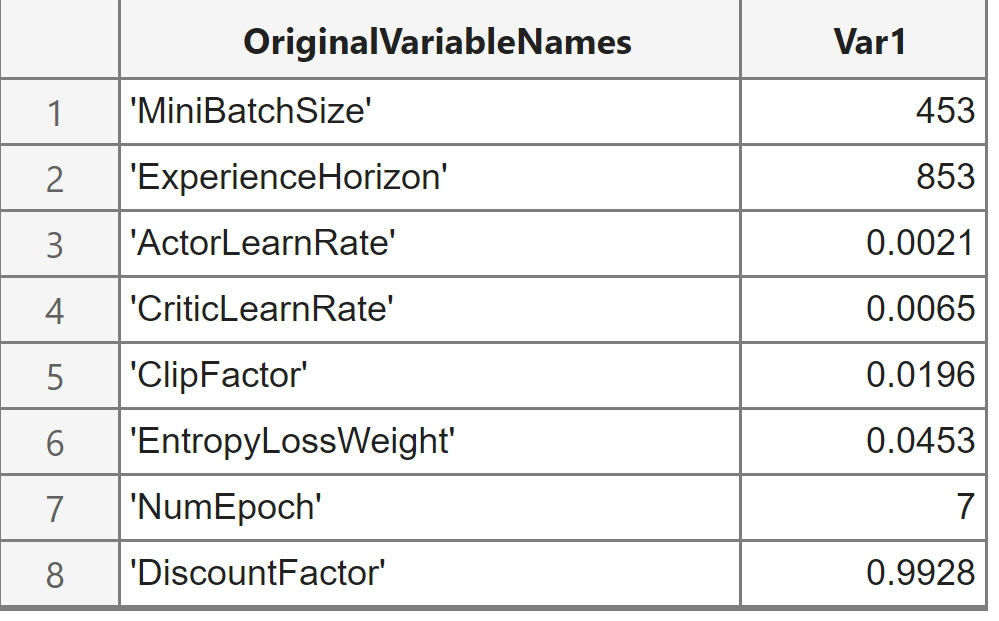
Retrieve the adjusted agent and training results stored in the UserDataTrace attribute. For convenience, the adjusted agent and training results can be loaded from disk.
if runOptimization % Get the optimized agent and results userData = optimResults.UserDataTrace{iteration}; tunedAgent = userData.Agent; tunedResult = userData.TrainingResult; else % Load previously optimized agent and results load("LanderOptimResults.mat","tunedAgent","tunedResult"); endView the training process of the optimized agent; due to the randomness of training, different results will be obtained during self-training.
show(tunedResult)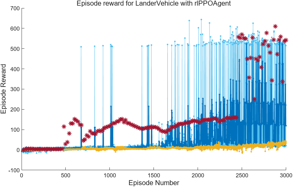
Simulating the optimized agent in the environment will not be elaborated upon here; interested readers can refer to the official documentation.
04
—
References
[1] Bayesian Optimization Algorithm
https://www.mathworks.com/help/stats/bayesian-optimization-algorithm.html
[2] Wang, J., Du, C., Yan, F., Duan, X., Hua, M., Xu, H., & Zhou, Q. (2024). Energy Management of a Plug-in Hybrid Electric Vehicle Using Bayesian Optimization and Soft Actor-Critic Algorithm. IEEE Transactions on Transportation Electrification.
https://ieeexplore.ieee.org/document/10522790
[3] Wang, J., Du, C., Yan, F., Hua, M., Gongye, X., Yuan, Q., … & Zhou, Q. (2025). Bayesian optimization for hyper-parameter tuning of an improved twin delayed deep deterministic policy gradients based energy management strategy for plug-in hybrid electric vehicles. Applied Energy, 381, 125171.
https://doi.org/10.1016/j.apenergy.2024.125171
[4] Tune Hyperparameters Using Bayesian Optimization
https://www.mathworks.com/help/releases/R2024b/reinforcement-learning/ug/tune-hyperparameters-using-bayesian-optimization.html?searchHighlight=bayesian%20reinforcement%20learning&s_tid=doc_srchtitle
[5] Optimize Cross-Validated Classifier Using bayesopt
https://www.mathworks.com/help/releases/R2024b/stats/bayesian-optimization-case-study.html
[6] Train PPO Agent for a Lander Vehicle
https://www.mathworks.com/help/releases/R2024b/reinforcement-learning/ug/train-ppo-agent-to-land-vehicle.html