Partial Least Squares (PLS) Regression Model in Matlab: Outlier Detection and Variable Selection

Full text download:http://tecdat.cn/?p=22319

This article establishes a Partial Least Squares (PLS) regression (PLSR) model and evaluates its predictive performance. To create a reliable model, we also implement several common outlier detection and variable selection methods to remove potential outliers and use a subset of selected variables to “clean” your data(Click the “Read the original text” at the end for the complete code data).

Related Videos

Steps

Establish the PLS regression model
K-fold cross-validation for PLS
Monte Carlo cross-validation (MCCV) for PLS.
Double cross-validation (DCV) for PLS
Outlier detection using Monte Carlo sampling method
Variable selection using the CARS method.
Variable selection using Moving Window PLS (MWPLS).
Variable selection using Monte Carlo Uninformative Variable Elimination (MCUVE)
Conduct variable selection

Establishing the PLS Regression Model

This example illustrates how to establish a PLS model using benchmark near-infrared data.

plot(X");               % Display spectral data.
xlabel('Wavelength Index');
ylabel('Intensity');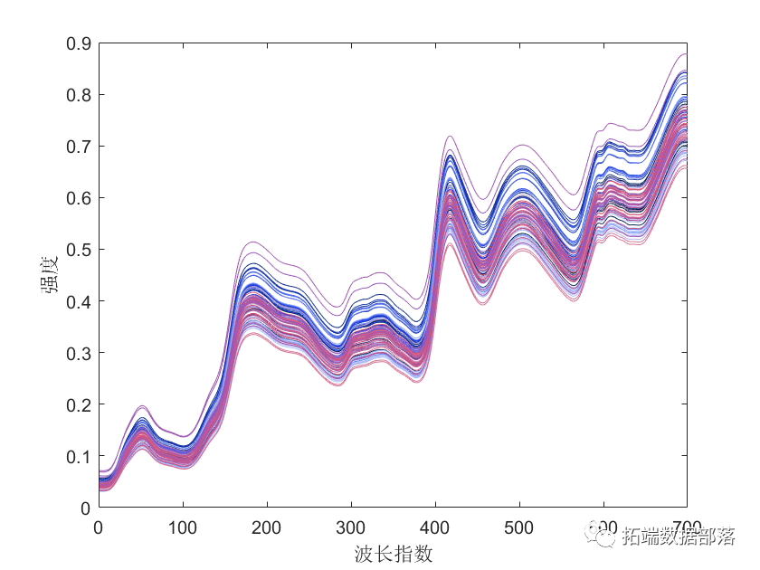

Parameter settings

A=6;                    % Number of latent variables (LV).
method='center';        % Internal preprocessing method for X to establish the PLS model
PLS(X,y,A,method);  % Command to establish the model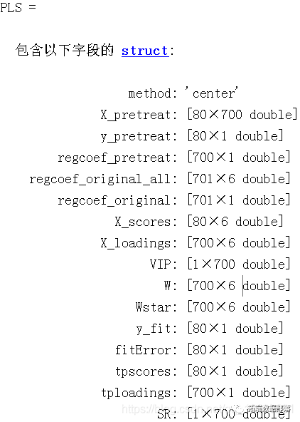

The pls.m function returns an object PLS containing a list of components. Result interpretation.

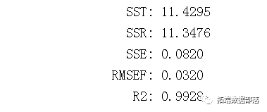
regcoef_original: Regression coefficients connecting X and y.X_scores: Scores of X.VIP: Variable Importance in Projection, a criterion for assessing variable importance.Importance of variables.RMSEF: Root Mean Square Error of Fit.y_fit: Fitted values of y.R2: Percentage of explained variation in Y.

K-Fold Cross-Validation for PLS

Describes how to perform K-fold cross-validation on the PLS model

clear;
A=6;                          % Number of LVs
K=5;                          % Number of cross-validation folds

plot(CV.RMSECV)               % Plot RMSECV values for each number of latent variables (LVs)
xlabel('Number of Latent Variables (LVs)')          % Add x label
ylabel('RMSECV')              % Add y label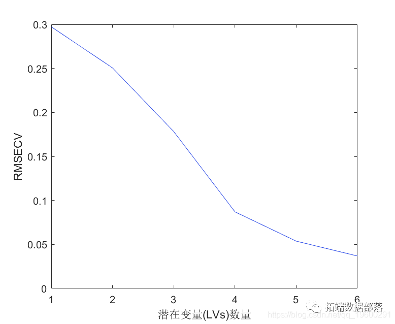

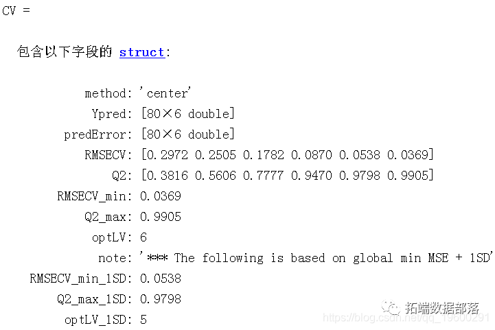
The returned value CV is a structured data with a list of components. Result interpretation.

RMSECV: Root Mean Square Error of Cross-Validation. The smaller, the better.Q2: Same meaning as R2, but calculated from cross-validation.optLV: Number of LVs that achieve minimum RMSECV (highest Q2).

Click the title to view related content

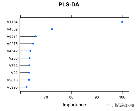
Partial Least Squares Regression PLS-DA in R

Swipe left to see more

Monte Carlo Cross-Validation (MCCV) for PLS

Describes how to perform MCCV for PLS modeling. Similar to K-fold CV, MCCV is another method of cross-validation.

Related Videos

% Parameter settings
A=6;
method='center';
N=500;                          % Number of Monte Carlo samples
% Run MCCV.
plot(MCCV.RMSECV);              % Plot RMSECV values for each number of latent variables (LVs)
xlabel('Number of Latent Variables (LVs)');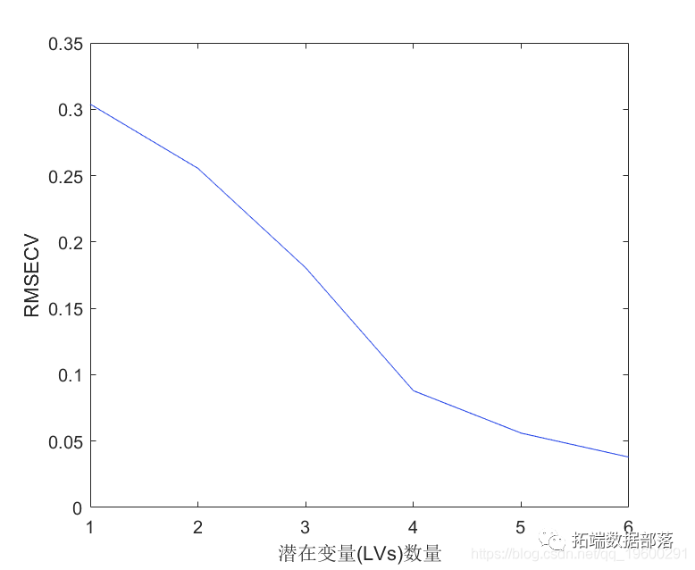

MCCV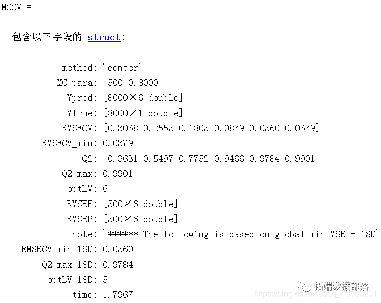

MCCV is a structured data. Result interpretation.

Ypred: Predicted valuesYtrue: True valuesRMSECV: Root Mean Square Error of Cross-Validation, the smaller, the better.Q2: Same meaning as R2, but calculated from cross-validation.

Double Cross-Validation (DCV) for PLS

Describes how to perform DCV for PLS modeling. Similar to K-fold CV, DCV is a method of cross-validation.

% Parameter settings

N=50;                                 % Number of Monte Carlo samples
dcv(X,y,A,k,method,N);
DCV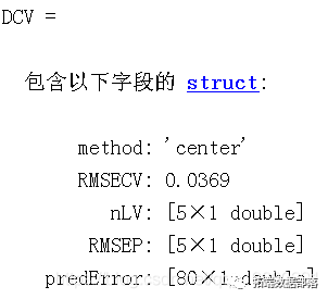

Outlier Detection Using Monte Carlo Sampling Method

Describes the usage of outlier detection methods

A=6;
method='center';
F=mc(X,y,A,method,N,ratio);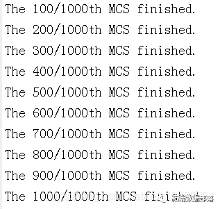

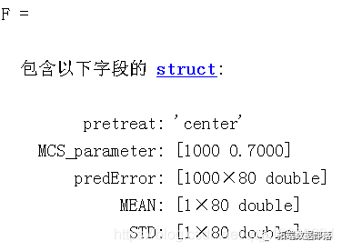
Result interpretation.

predError: Prediction error for each sample in the samplingMEAN: Average prediction error for each sampleSTD: Standard deviation of prediction error for each sample

plot(F) % Diagnostic plot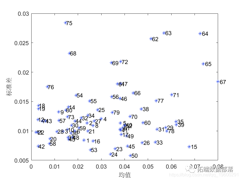

Note: Samples with high MEAN or SD values are more likely to be outliers and should be considered for removal before modeling.

Variable Selection Using the CARS Method.

A=6;
fold=5;
car(X,y,A,fold);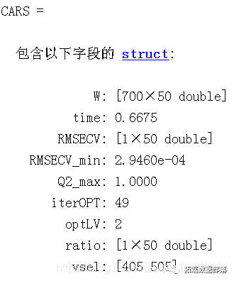

Result interpretation.

optLV: Number of LVs for the best modelvsel: Selected variables (columns in X).

plotcars(CARS); % Diagnostic plot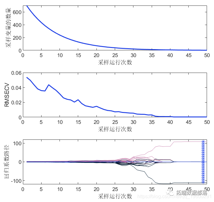

Note: In this figure, the top and middle panels show how the number of selected variables and RMSECV change with iterations. The bottom panel describes how the regression coefficients of each variable (each line corresponds to one variable) change with iterations. The star vertical line indicates the best model with the lowest RMSECV.

Variable Selection Using Moving Window PLS (MWPLS)

load corn_m51;                      % Example data
width=15;                           % Window size
mw(X,y,width);
plot(WP,RMSEF);
xlabel('Window Position');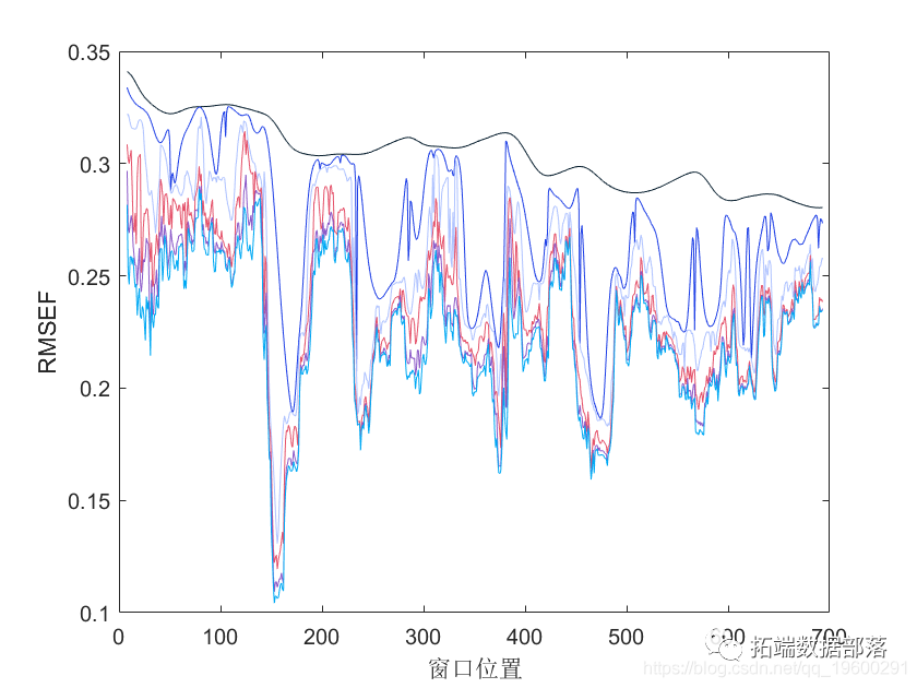

Note: The graph suggests including areas with lower RMSEF values into the PLS model.

Variable Selection Using Monte Carlo Uninformative Variable Elimination (MCUVE)

N=500;
method='center';

UVE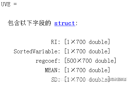

plot(abs(UVE.RI))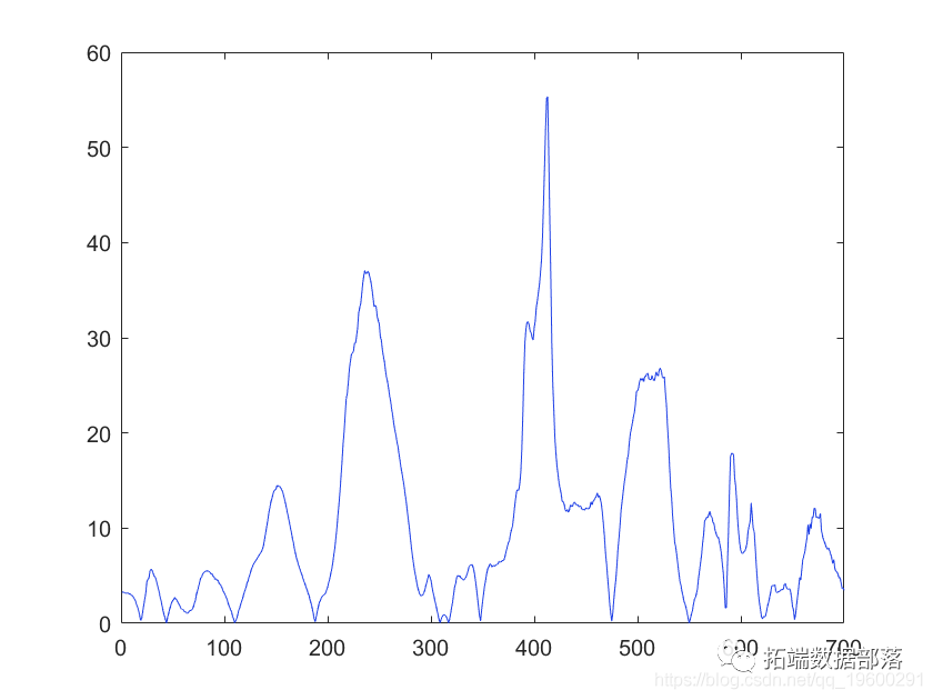

Result interpretation. RI: Reliability Index of UVE, a measure of variable importance, the higher, the better.

Conduct Variable Selection

A=6;
N=10000;
method='center';
FROG=rd_pls(X,y,A,method,N);


              N: 10000
              Q: 2
          model: \[10000x700 double\]
        minutes: 0.6683
         method:'center'
          Vrank: \[1x700 double\]
         Vtop10: \[505405506400408233235249248515\]
    probability: \[1x700 double\]
           nVar: \[1x10000 double\]
          RMSEP: \[1x10000 double\]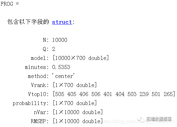

xlabel('Variable Index');
ylabel('Selection Probability');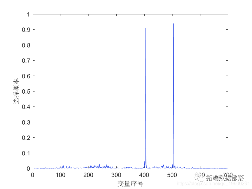

Result interpretation:

The model result is a matrix that stores the selected variables in each relationship.Probability: The probability of each variable being included in the final model. The larger, the better. This is a useful indicator of variable importance.

This article shares the analyzed data and code in the member group, scan the QR code below to join the group!

This excerpt from《Partial Least Squares (PLS) Regression Model in Matlab: Outlier Detection and Variable Selection》, click “Read the original text” to obtain the complete data.

Click the title to view past content

Implementation of Partial Least Squares (PLS) Regression in R Block Gibbs Sampling Bayesian Multivariate Linear Regression in RImplementation of Lasso Regression Model Variable Selection and Diabetes Development Prediction Model in RImplementation of Bayesian Quantile Regression, Lasso and Adaptive Lasso Bayesian Quantile Regression Analysis in RBayesian Regression Analysis of Housing Affordability Dataset in PythonImplementation of Bayesian Linear Regression Model with PyMC3 in PythonInterval Data Regression Analysis in RTime Series Anomaly Detection Using LOESS (Locally Weighted Regression) Seasonal Trend Decomposition (STL) in RAnalysis of Economic Time Series Using Time-Varying Markov Regime Switching (MRS) Autoregressive Model in PYTHONRandom Forest, Logistic Regression to Predict Heart Disease Data and Visualization Analysis in RImplementation of LASSO Regression Analysis Based on RImplementation of Bayesian Linear Regression Model with PyMC3 in PythonPolynomial Regression, Nonlinear Regression Model Curve Fitting Using RPLS-DA in REcological Modeling in R: Boosted Regression Trees (BRT) Predicting Shortfin Mako Shark Survival Distribution and Influencing FactorsImplementation of Partial Least Squares (PLS) Regression in RPartial Least Squares Regression (PLSR) and Principal Component Regression (PCR)How to Find Differentiated Indicators in Patient Data? (PLS-DA Analysis) in R