Introduction to Quantitative Investment with Python: Build Your First Trading Strategy from Scratch

1. What is Quantitative Investment?

Quantitative Investment refers to a trading method that issues buy and sell orders through quantitative means and computer programming, aiming to achieve excess returns or a specific risk-return ratio. It leverages modern statistics and mathematical methods, utilizing computer technology to find “high probability” strategies and patterns from vast historical data that can yield excess returns, and executes investment ideas according to these strategies through a disciplined quantitative model.

The core advantages are:

• Discipline: Avoids emotional decision-making errors by investors during market fluctuations.

• Efficiency: Can monitor multiple markets and assets simultaneously, capturing more trading opportunities.

• Verifiability: Validates the effectiveness of strategies through historical data backtesting.

• Timeliness: Quickly processes large amounts of data, tracks market dynamics in real-time, and captures trading signals promptly.

2. Why Choose Python?

Python has become a popular language for quantitative investment due to its rich financial libraries and simple syntax. Here are commonly used Python quantitative investment toolchains:

• Data Acquisition Tools:

• Tushare: A free and open-source financial data interface that provides market data for stocks, funds, futures, etc.

• AkShare: A financial data interface covering multiple fields such as stocks, futures, foreign exchange, and digital currencies.

• yfinance: Fetches data from Yahoo Finance.

• Financial Data Platform APIs: Python APIs from platforms like Wind and Tonghuashun, providing real-time and historical data.

• Data Processing and Analysis Libraries:

• pandas: Provides high-performance data structures and data analysis tools.

• NumPy: Supports large-scale multi-dimensional array and matrix operations.

• TA-Lib: A technical analysis library that provides calculation functions for hundreds of technical indicators.

• Quantitative Trading Frameworks:

• Zipline: An open-source backtesting framework developed by Quantopian, supporting custom data sources and complex trading logic.

• VN.PY: A popular open-source quantitative trading framework in China, supporting real trading for stocks, futures, options, etc.

• Backtrader: A lightweight backtesting framework that supports multiple markets and data sources.

• Trade Execution Tools:

• Easytrader: An automated stock trading interface that supports multiple brokers.

• RiceQuant: Provides a one-stop solution for strategy development, historical backtesting, and simulated trading.

3. Environment Setup

Use pip to install the relevant libraries.

pip install pandas numpy tushare matplotlib backtrader

4. Data Acquisition and Processing

4.1. Data Acquisition

Using Tushare as an example, to acquire historical price data for stocks:

import tushare as ts
# Initialize Tushare (register to get token)
ts.set_token('YOUR_API_TOKEN')
pro = ts.pro_api()
# Get historical market data for Industrial and Commercial Bank of China (601398.SH)
df = pro.daily(ts_code='601398.SH', start_date='20240601', end_date='20250422')
print(df.head())

Note:

• The ts.set_token() method is used to initialize Tushare and set the API Token. Please register an account on the Tushare website to obtain the token and keep it secure.

• The pro=ts.pro_api() method creates an instance of the Tushare Pro API, which provides richer data interfaces and supports more complex queries.

• The pro.daily() method is used to obtain historical market data for stocks.

4.2. Data Preprocessing

Clean and preprocess the acquired data:

import pandas as pd
# Convert trade_date column to datetime format
df['trade_date'] = pd.to_datetime(df['trade_date'])
# Sort by date
df = df.sort_values(by='trade_date', ascending=True)
# Set index
df.set_index('trade_date', inplace=True)
# Calculate returns
df['returns'] = df['close'].pct_change()
# Fill missing values (using the previous day's closing price)
df.fillna(method='ffill', inplace=True)
# Print open price, close price, returns
print(df[['open', 'close', 'returns']].tail())

Note:

• The pd.to_datetime() method is used to convert the data type of the column (string or number) to datetime format.

• The sort_values() method is used to sort by the specified column, with ascending=True indicating ascending order (from smallest to largest).

• The set_index() method is used to set the index of the DataFrame, with inplace=True indicating that the original DataFrame is modified directly. After setting the date index, data can be accessed quickly by date.

• The pct_change() method is used to calculate the daily return of the closing price. It subtracts the previous row’s value from the current row’s value, divides by the previous row’s value, and finally multiplies by 100 to get the percentage growth rate.

5. Building a Trading Strategy

5.1. Strategy Design: Moving Average Crossover Strategy

Strategy Logic:

• Calculate short-term (e.g., 10-day) and long-term (e.g., 50-day) moving averages.

• When the short-term moving average crosses above the long-term moving average, a buy signal is generated; when it crosses below, a sell signal is generated.

5.2. Strategy Implementation

# Calculate moving averages
df['SMA_10'] = df['close'].rolling(window=10).mean()        # 10-day moving average
df['SMA_20'] = df['close'].rolling(window=20).mean()        # 20-day moving average
df['SMA_30'] = df['close'].rolling(window=30).mean()        # 30-day moving average
# Generate trading signals (avoid lookahead bias, signals lag by one period)
# When the short-term moving average crosses above the long-term moving average, generate a buy signal; when it crosses below, generate a sell signal.
df['Signal'] = np.where(df['SMA_10'] > df['SMA_20'], 1, np.where(df['SMA_10'] < df['SMA_20'], -1, 0))
df['Signal'] = df['Signal'].shift(1)
# Calculate strategy returns
df['Strategy_Returns'] = df['Signal'] * df['returns']
# Calculate cumulative returns
df['Cumulative_Returns'] = (1 + df['Strategy_Returns']).cumprod()
print(df[['close', 'SMA_10', 'SMA_20', 'Signal', 'Strategy_Returns', 'Cumulative_Returns']].tail(100))

Note:

1. Calculate moving averages

• rolling(window=10) is used to create a rolling window object with a size of 10.

• .mean() is used to calculate the average of the closing prices within the window, resulting in the 10-day moving average (SMA_10).

2. Generate trading signals. Generate trading signals based on the crossover of moving averages.

• When the 10-day moving average (SMA_10) crosses above the 20-day moving average (SMA_20), set Signal to 1 (buy signal).

• When the 10-day moving average crosses below the 20-day moving average, set Signal to -1 (sell signal).

• shift(1): Lags the signal by one period to ensure that trading signals are generated based on historical data, avoiding the use of future data.

3. Calculate strategy returns

• When Signal is 1 (buy signal), the strategy return equals the daily return.

• When Signal is -1 (sell signal), the strategy return equals the negative of the daily return (assuming short selling).

• When Signal is 0 (no signal), the strategy return is 0.

4. Calculate cumulative returns

• (1 + df[‘Strategy_Returns’]): Converts strategy returns to growth rates (e.g., a return of 5% results in a growth rate of 1.05).

• .cumprod(): Calculates the cumulative product, resulting in the cumulative return curve of the strategy.

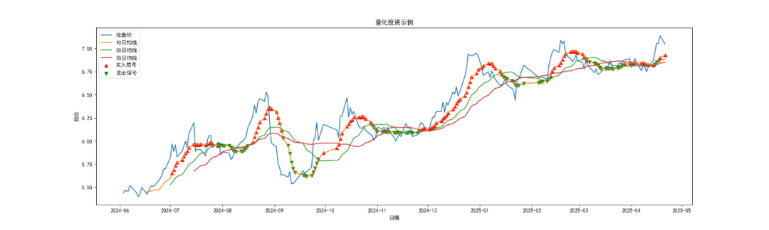
6. Visualization

import matplotlib.pyplot as plt
from matplotlib import rcParams
# Set font to SimHei to support Chinese display
rcParams['font.sans-serif'] = ['SimHei']  # Use black body font
rcParams['axes.unicode_minus'] = False    # Solve the issue of negative sign '-' displaying as a square
# Plot cumulative return curve
plt.figure(figsize=(20, 6))                         # Create a new figure window
plt.plot(df['close'], label='Close Price')          # Plot close price curve
plt.plot(df['SMA_10'], label='10-Day MA')       # Plot 10-day moving average curve
plt.plot(df['SMA_20'], label='20-Day MA')       # Plot 20-day moving average curve
plt.plot(df['SMA_30'], label='30-Day MA')       # Plot 30-day moving average curve
# Mark buy and sell signals
plt.scatter(df[df['Signal'] == 1].index, df[df['Signal'] == 1]['SMA_10'], marker='^', color='r', label='Buy Signal')
plt.scatter(df[df['Signal'] == -1].index, df[df['Signal'] == -1]['SMA_10'], marker='v', color='g', label='Sell Signal')
plt.title("Quantitative Investment Example")
plt.xlabel("Date")
plt.ylabel("Stock Price")
plt.legend()
plt.show()

Note:

• Set font to solve Chinese display issues.

• Set font to SimHei (black body) to ensure proper display of Chinese characters.

• Set axes.unicode_minus=False to solve the issue of negative signs displaying as squares.

• Create figures and axes.

• Create a new figure window, setting the figure size to 20 x 6 inches to ensure the chart is wide enough to display time series data.

• Plot data curves.

• df[‘close’]: Stock close price curve.

• df[‘SMA_10’]: 10-day moving average.

• The label parameter names each curve for later legend display.

• Mark buy and sell signals.

• df[df[‘Signal’] == 1].index: Filters out dates where Signal is 1 (buy signal).

• df[df[‘Signal’] == 1][‘SMA_10’]: Gets the 10-day moving average values corresponding to those dates.

• marker=’^’: Marks buy signals with red triangles (^).

• marker=’v’: Marks sell signals with green inverted triangles (v).

• Set chart title, axis labels, and legend.

• plt.title(): Sets the chart title to “Quantitative Investment Example”.

• plt.xlabel(): Sets the x-axis label to “Date”.

• plt.ylabel(): Sets the y-axis label to “Stock Price”.

• plt.legend(): Displays the legend, explaining the meaning of each curve and marker.

• Display the chart.

• plt.show() is used to render and display the chart.

Effect:

7. Strategy Backtesting and Evaluation

7.1. Return Analysis

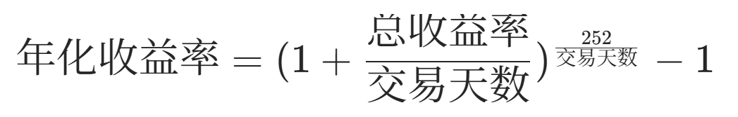
total_return = (df['Cumulative_Returns'].iloc[-1] - 1) * 100
annualized_return = (1 + total_return / len(df)) ** (252 / len(df)) - 1  # Assuming 252 trading days per year
print(f"Total Return: {total_return:.2f}%")
print(f"Annualized Return: {annualized_return:.2f}")

Note:

• Total Return. The first line of code calculates the cumulative return of the strategy over the entire backtesting period.

• df[‘Cumulative_Returns’].iloc[-1]: Gets the last value of the cumulative return column (i.e., the final cumulative return).

• -1: Converts cumulative return to a ratio relative to the initial investment (e.g., a cumulative return of 1.5 indicates a 50% increase).

• * 100: Converts the ratio to percentage form.

• Annualized Return. The second line of code calculates the annualized return based on total return, reflecting the long-term profitability of the strategy.

• len(df): Gets the number of data points (i.e., trading days).

• 252: Assuming there are 252 trading days in a year.

• Formula:

  

7.2. Risk Assessment

# Calculate maximum drawdown
df['Peak'] = df['Cumulative_Returns'].cummax()
df['Drawdown'] = (df['Peak'] - df['Cumulative_Returns']) / df['Peak']
max_drawdown = df['Drawdown'].max()
# Calculate Sharpe Ratio (assuming risk-free return is 0)
mean_return = df['Strategy_Returns'].mean() * 252  # Annualized average return
std_return = df['Strategy_Returns'].std() * np.sqrt(252)  # Annualized return standard deviation
sharpe_ratio = mean_return / std_return
print(f"Maximum Drawdown: {max_drawdown:.2f}")
print(f"Sharpe Ratio: {sharpe_ratio:.2f}")

Note:

• Maximum Drawdown: The maximum potential loss the strategy may face during the backtesting period.

• Peak: Calculates the maximum value sequence of cumulative returns.

• cummax(): Calculates the maximum cumulative return along the time axis.

• Drawdown: Calculates the drawdown ratio from the peak to the current value. Formula: Drawdown = (Peak – Current Value) / Peak

• Maximum Drawdown: Gets the maximum value of the drawdown ratio, reflecting the maximum potential loss the strategy may face during the backtesting period.

• Sharpe Ratio: Measures risk-adjusted returns; a higher value indicates a better cost-performance ratio of the strategy.

• Annualized Average Return: Calculates the mean of the strategy return column and multiplies by 252 to get the annualized average return.

• Annualized Return Standard Deviation: Calculates the standard deviation of the strategy return column and multiplies by 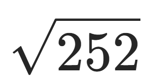to get the annualized return standard deviation.

• Sharpe Ratio: Calculates risk-adjusted returns. Formula: Sharpe Ratio = Annualized Average Return / Annualized Return Standard Deviation.

• The larger the Sharpe Ratio, the better the cost-performance ratio of the strategy.

8. Strategy Optimization and Iteration

• Parameter Optimization: Adjust the periods of moving averages (e.g., try combinations of 5-day, 20-day, and 60-day moving averages) to find the best parameter combination.

• Strategy Fusion: Combine the moving average strategy with other strategies (e.g., RSI overbought/oversold strategy) to enhance strategy stability.

• Risk Management: Incorporate stop-loss and take-profit mechanisms to control the maximum loss and profit of each trade.

9. Conclusion

Through the above steps, you have completed the construction, backtesting, and evaluation of a simple quantitative investment trading strategy. Quantitative investment is a continuous learning and iteration process, and you need to constantly:

• Optimize Strategies: Adjust strategy logic and parameters based on market changes.

• Expand Data Sources: Introduce alternative data (e.g., social media sentiment, satellite images) to enhance strategy predictive capabilities.

• Strengthen Risk Control: Improve risk management measures to ensure the robustness of strategies in different market environments.

Next Steps Recommendations:

• Use tools like Tushare to obtain real market data, replacing the simulated data in the examples.

• Try deploying strategies in quantitative trading frameworks (like Zipline, VN.PY) for more complex backtesting and live trading.

• Learn machine learning algorithms (e.g., random forests, LSTM neural networks) to explore machine learning-based quantitative strategies.