
MATLAB Visualization of Spatial Distribution of Correlation Coefficients

Author: Eighth Galaxy – Stone Man
Contact Email: [email protected]
Data:ERA5 Data
Read Data
*%% Spatial Distribution of Correlation Coefficients
clc;clear;close all

%% Read Data
path = "E:\z\hhh.nc";    % Set data file path
ncdisp(path)     % Display variables and their precision in the data file
mlat = double(ncread(path,'latitude'));   % Latitude
mlon = double(ncread(path,'longitude'));  % Longitude
[nlat,nlon]=meshgrid(mlat,mlon);   % Convert vector to matrix
t = double(ncread(path,'t2m'));   % Temperature variable
r = double(ncread(path,'sro'));   % Runoff variable

sjyData = readmatrix('E:\z\hhh.txt');   % Area range
VarName1 = sjyData(:,1)';    % Area longitude
VarName2 = sjyData(:,2)';    % Area latitude

lat = reshape(nlat,57*29,1);    % Convert matrix to vector for scatter plot
lon = reshape(nlon,57*29,1);    % 57 and 29 represent the number of rows and columns of the original data
Process Data
%% Process Data
% Calculate correlation (corrcoef function)
% Relationship between variable t and variable r
cor1t = zeros(1,1);     % Define new matrix
cor2t = zeros(57,29);
cor3t = zeros(57,29);
for i = 1:57     % Loop to calculate the correlation for each point, R represents correlation, P is the significance test result
    for j = 1:29
        for k = 1:252
            cor1t(k,1) = t(i,j,k);
            cor1t(k,2) = r(i,j,k);
        end
        [R,P] = corrcoef(cor1t);
        cor2t(i,j) = R(1,2);
        cor3t(i,j) = P(1,2);
    end
end

% Check if it passes the significance test (P<0.01)
cor4t = zeros(57,29);
for i = 1:57
    for j = 1:29
        if cor3t(i,j)>=0.01
           cor4t(i,j) = NaN;
        elseif cor3t(i,j)<0.01
            cor4t(i,j) = cor3t(i,j);
        end
    end
end

% Filter the required area (inpolygon function)
for i = 1:57
    for j = 1:29
        GZs = inpolygon(nlon(i,j),nlat(i,j),VarName1,VarName2);
        if GZs == 0
            cor2t(i,j) = NaN;
            cor4t(i,j) = NaN;
        end
    end
end
cor4t(isnan(cor4t) ~= 1) = 1;
cor5t = reshape(cor4t,57*29,1);
Plotting
%% Plotting
figure('position',[200,5,600,300])   % Set figure position and size
m_proj('miller','lon',[89 103],'lat',[31 38]);  % Set projection type
m_contourf(nlon,nlat,cor2t,'linestyle','none');  % Fill color for correlation coefficients
hold on
m_plot(VarName1,VarName2,'k','linewidth',1);  % Draw area boundary
hold on;
shading interp;
hold on
m_scatter(lon,lat,cor5t,'k','linewi',1)    % Significant test points
hold on
m_grid('linestyle','none');    % Set grid
hold off
colorbar
colormap(nclCM(382))    % nclCM is a function from the colormap package
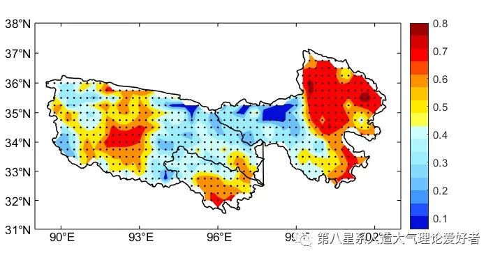
Reference Image
Complete Code
%% Spatial Correlation Plotting
clc;clear;close all
%% Read Data
path = "E:\z\hhh.nc"; % Set data file path
ncdisp(path) % Display variables and their precision in the data file
mlat = double(ncread(path,'latitude')); % Latitude
mlon = double(ncread(path,'longitude')); % Longitude
[nlat,nlon]=meshgrid(mlat,mlon); % Convert vector to matrix
t = double(ncread(path,'t2m')); % Temperature variable
r = double(ncread(path,'sro')); % Runoff variable
sjyData = readmatrix('E:\z\hhh.txt'); % Area range
VarName1 = sjyData(:,1)'; % Area longitude
VarName2 = sjyData(:,2)'; % Area latitude
lat = reshape(nlat,57*29,1); % Convert matrix to vector for scatter plot
lon = reshape(nlon,57*29,1); % 57 and 29 represent the number of rows and columns of the original data
%% Process Data
% Calculate correlation (corrcoef function)
% Relationship between variable t and variable r
cor1t = zeros(1,1); % Define new matrix
cor2t = zeros(57,29);
cor3t = zeros(57,29);
for i = 1:57 % Loop to calculate the correlation for each point, R represents correlation, P is the significance test result
for j = 1:29
for k = 1:252
cor1t(k,1) = t(i,j,k);
cor1t(k,2) = r(i,j,k);
end
[R,P] = corrcoef(cor1t);
cor2t(i,j) = R(1,2);
cor3t(i,j) = P(1,2);
end
end
% Check if it passes the significance test (P<0.01)
cor4t = zeros(57,29);
for i = 1:57
for j = 1:29
if cor3t(i,j)>=0.01
cor4t(i,j) = NaN;
elseif cor3t(i,j)<0.01
cor4t(i,j) = cor3t(i,j);
end
end
end
% Filter the required area (inpolygon function)
for i = 1:57
for j = 1:29
GZs = inpolygon(nlon(i,j),nlat(i,j),VarName1,VarName2);
if GZs == 0
cor2t(i,j) = NaN;
cor4t(i,j) = NaN;
end
end
end
cor4t(isnan(cor4t) ~= 1) = 1;
cor5t = reshape(cor4t,57*29,1);
%% Plotting
figure('position',[200,5,600,300]) % Set figure position and size
m_proj('miller','lon',[89 103],'lat',[31 38]); % Set projection type
m_contourf(nlon,nlat,cor2t,'linestyle','none'); % Fill color for correlation coefficients
hold on
m_plot(VarName1,VarName2,'k','linewidth',1); % Draw area boundary
hold on;
shading interp;
hold on
m_scatter(lon,lat,cor5t,'k','linewi',1) % Significant test points
hold on
m_grid('linestyle','none'); % Set grid
hold off
colorbar
colormap(nclCM(382)) % nclCM is a function from the colormap package
% For details see the link
%https://blog.csdn.net/slandarer/article/details/127935365?ops_request_misc=&request_id=&biz_id=102&utm_term=ncl%E8%89%B2%E5%8D%A1%E7%94%A8%E4%BA%8Ematlab&utm_medium=distribute.pc_search_result.none-task-blog-2~all~sobaiduweb~default-5-127935365.nonecase&spm=1018.2226.3001.4187

Sent from the backend:Group chat QR code,
Join the group chat by sending this code,
Daily data sharing in the group
Editor: Zhi Zhi