MATLAB Plotting Techniques | 3D Line Plot (With Code)

3D data visualization provides learners with intuitive images and is widely used. The previous post mainly introduced 3D surface plotting, involving functions such as meshgrid, mesh, meshc, surf, surfl, and surfc.

The 3D line plot aims to showcase the curve distribution in three-dimensional space and uses the MATLAB function plot3. The difference from the 2D line plotting function plot is that you need to set the x, y, and z coordinate vectors, while other plotting attributes are basically the same. Similar functions include the 3D scatter plot scatter3, and the 3D stem plot stem3.

Below, we use Fourier series expansion for 3D visualization as a code example.

clc; clear; close all;

%———————-

m = 15; % Series

N = 512; % Period

T0 = 4;

T = 2;

t1 = linspace(-T/2, T/2, N);

t2 = linspace(T/2, T0-T/2, N);

t = [(t1-T0)’; (t2-T0)’; t1′; t2′; (t1+T0)’];

%———————-

% Construct periodic signals

%———————-

% s = zeros(5*N,1);

% s(1:N)=1; s(2*N+1:3*N)=1; s(4*N+1:5*N)=1;

s = [ones(N,1);zeros(N,1);ones(N,1);zeros(N,1);ones(N,1)]’;

y = zeros(m+1, length(s));

y(m+1,:) = s-0.5;

plot3(t-(t+2), t, y(m+1,:),‘LineWidth’,2); % Period square wave

hold on;

axis([-2,m+1,-T0-1,T0+1,-1,2])

set(gca,‘XTick’,-T0-1:2:m);

set(gca,‘YTick’,-T0-1:1:T0+1);

set(gca,‘ZTick’,-1:0.5:T0);

title(‘Fourier series expansion’,‘FontSize’,15);

grid on;

view(-49,23)

fsamp = 1028;

f = linspace(1, m+1, fsamp);

A = 0.5; % Coefficient

freq = 1:1:m;

plot3(f,T0+f-f+1,A*sinc(A*f)*5,‘LineWidth’,3)

mag = A*sinc(A*freq)*5;

h=stem3(freq,T0+freq-freq+1,mag,‘filled’,‘LineWidth’,3);

set(h,‘Marker’,‘o’,‘MarkerFaceColor’,‘g’)

x = A*ones(size(t));% Harmonic signals

X = A*ones(size(t));% Synthesis signals

for k = 1:m

x = 2*A*sinc(A*k)*cos(2*pi*t*k/T0);

X = X+2*A*sinc(A*k)*cos(2*pi*t*k/T0);

y(k, 🙂 = x;

plot3(k+t-t, t, y(k,:),‘LineWidth’,1.5); % Harmonic

end

plot3(k+1+t-t, t, X-0.5,‘LineWidth’,2);

grid on;

xlabel(‘Frequency view’,‘Rotation’, 15);

ylabel(‘Time duration’,‘Rotation’, -10);

zlabel(‘Amplitude/Magnitude’);

set(gcf,‘Color’,‘White’); % Background is white

%———————-

The program runs as shown in Figure B6-1.

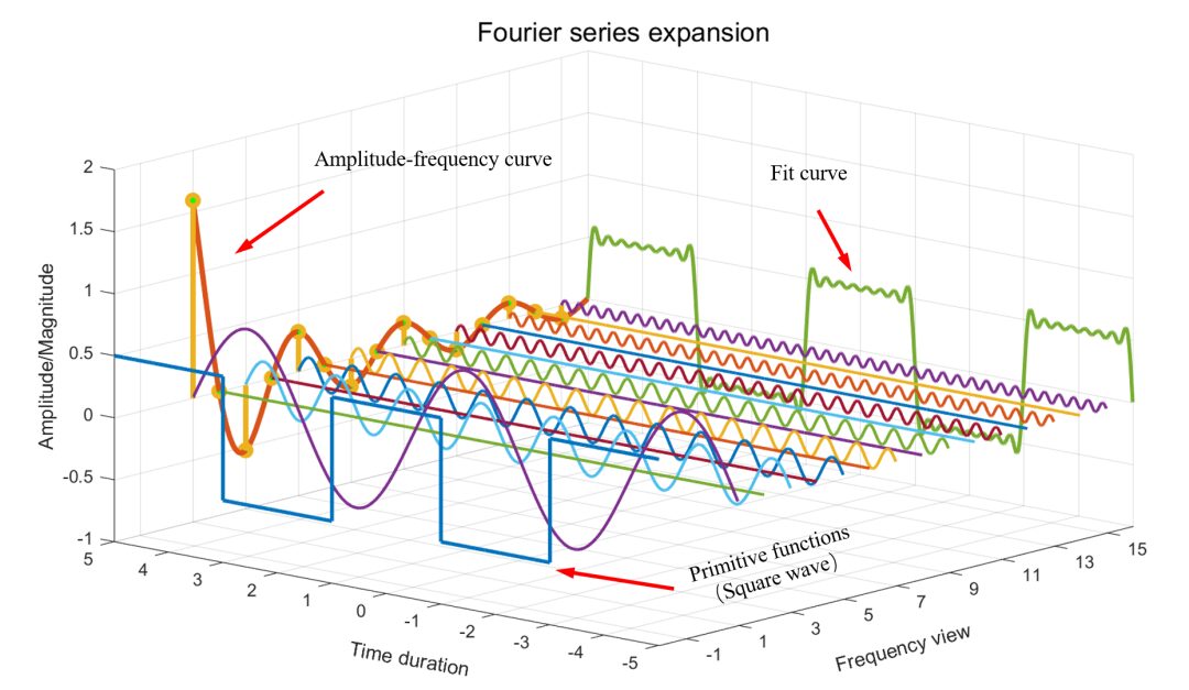
Figure B6-1 3D visualization of Fourier series expansion

Here are some useful public accounts for algorithms and scientific research plotting:

Image credit:Peng Zhenming

Editor: HuChenChen

Previous

Issues

Review

Summary

MATLAB Plotting Techniques | 3D Surface (With Code)

MATLAB Plotting Techniques | DIY Music Player (With Code)

MATLAB Plotting Techniques | Polygon Area Filling Plot (With Code)

MATLAB Plotting Techniques | Color Gradient Line Plot (With Code)

MATLAB Plotting Techniques | Line Plot (With Code)

MATLAB Plotting Techniques | Color Gradient Bar Plot

Congratulations! Master’s student Han Yaqi from IDIP Laboratory published research results in IEEE TGRS

Congratulations! Master’s student Wang Guanghui from IDIP Laboratory published research results in IEEE TGRS

Congratulations! Master’s student Cao Zhaoyang from IDIP Laboratory published a paper in a top journal in Zone 1

Sharing stories, discussing education topics, talking about life experiences, and writing warm words