1. Initial Impressions of Simscape Solver

In today’s simulation field, Simscape shines like a brilliant star, widely used in key industries such as automotive, aerospace, and industrial automation due to its excellent capabilities in multi-domain physical system modeling and simulation. Whether for precise simulation of complex mechanical systems, performance analysis of electronic circuits, or dynamic studies of hydraulic and pneumatic systems, Simscape demonstrates powerful functions that help engineers and researchers efficiently complete important tasks such as system design, optimization, and fault diagnosis.

In the entire process of Simscape simulation, the solver undoubtedly occupies a core position; it acts like a “behind-the-scenes hero” in the simulation world. Once we construct a sophisticated system model in Simscape, the solver begins to showcase its skills, solving the mathematical equations that describe the system’s behavior through a series of complex and ingenious algorithms, thus presenting the system’s dynamic response under different conditions. It is not an exaggeration to say that the performance of the solver directly affects the accuracy, reliability, and efficiency of the simulation results. Today, we will delve into the unique solver known as the Local Solver in Simscape.

2. What is Local Solver

Local Solver, as the name suggests, is a key component of the Simscape simulation solving system, primarily used to handle numerical computation tasks within the physical networks of models. In complex multi-domain physical system models built in Simscape, each physical network has its unique mathematical equations, and the Local Solver is responsible for accurately solving these equations to reveal the system’s state at different moments.

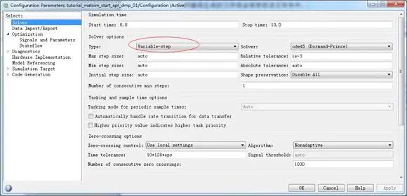
Compared to other solvers, the Local Solver has distinct characteristics. It is a fixed-step solver, which advances calculations using a pre-set fixed time step throughout the simulation process. This differs from variable-step solvers, which dynamically adjust the step size based on error conditions during the simulation process. The fixed-step nature of the Local Solver allows it to demonstrate unique advantages when dealing with systems that require high stability in time steps, ensuring the reliability and consistency of simulation results.

In the solving system of Simscape, the Local Solver plays an indispensable role. While the global solver (such as the Simulink solver) manages the overall simulation process and coordinates data interactions between different modules, the Local Solver focuses on in-depth processing of detailed calculations for each physical network. To put it metaphorically, the global solver is like the conductor of a large symphony orchestra, coordinating the overall performance; while the Local Solver is akin to the principal musicians of each instrument group, focusing on their respective performances, both working together to contribute to the successful operation of the simulation.

3. Characteristics of Local Solver

3.1 Stability

In the simulation world of Simscape, stability is one of the key indicators for measuring solver performance, and the Local Solver excels in this regard, largely due to its unique Backward Euler solving method. Backward Euler, as an implicit numerical solving method, shows strong oscillation suppression capability when dealing with ordinary differential equations.

For example, in a simple RLC circuit simulation, the interaction between inductors, capacitors, and resistors can easily produce oscillation phenomena due to the changes in current and voltage. When we use the Backward Euler solving method of the Local Solver for simulation, it cleverly handles the relationship between variables at the current moment and the next moment, effectively suppressing such oscillations. Mathematically, the Backward Euler method uses the unknown solution value at the next time point to approximate the derivative during iterative calculations, resulting in smoother calculation outcomes and avoiding severe fluctuations that may arise from changes in step size. Even during the simulation process, if external factors cause changes in the time step, such as when simulating the sudden connection or disconnection of a load in a circuit, the Backward Euler solving method can still maintain stable calculations, ensuring the reliability of simulation results. This stability makes the Local Solver one of the preferred solvers for engineers when dealing with oscillation-sensitive systems.

3.2 Oscillation Capture Capability

In certain specific simulation scenarios, we not only need to suppress oscillations but also need to accurately capture oscillation phenomena within the system for in-depth analysis of its dynamic characteristics. At this point, the Trapezoidal solving method within the Local Solver demonstrates its unique advantages.

The Trapezoidal method is based on the trapezoidal rule for numerical integration, and it can capture oscillation details more accurately than some other methods when dealing with oscillatory signals. We can intuitively demonstrate this advantage through a simulation experiment of a mechanical vibration system. In this mechanical vibration system, a mass block is connected between a spring and a damper, and when the system is subjected to external excitation, the mass block generates complex vibrations, with its displacement and velocity signals containing rich oscillation information. When we simulate using the Trapezoidal solving method and other common solving methods, it is evident that the Trapezoidal method can more clearly depict the oscillatory waveforms of displacement and velocity signals, accurately capturing changes in frequency and amplitude of oscillations. This is because the Trapezoidal method provides a more precise approximation of the integral of the signal during calculations, allowing for better fitting of the oscillatory signal’s curve. When analyzing systems that require precise knowledge of oscillation characteristics, such as audio signal processing systems or earthquake simulation systems, the oscillation capture capability of the Trapezoidal solving method can provide engineers and researchers with more valuable information, helping them gain deeper insights into system behavior for more effective system design and optimization.

3.3 Real-time Simulation Speed Improvement

In modern simulation applications, especially in scenarios with high real-time requirements, such as hardware-in-the-loop testing and real-time control system simulations, the speed of simulation directly impacts the overall performance and application effectiveness of the system. The Partitioning solving method in the Local Solver provides an effective way to enhance real-time simulation speed.

The core principle of Partitioning is to divide the entire set of equations corresponding to the Simscape network into a series of smaller sets of equations. In a complex power system simulation model, which contains numerous generators, transformers, transmission lines, and other components, the corresponding set of equations is large and complex. The Partitioning solving method will reasonably divide these sets of equations into multiple smaller equation modules based on the network’s structure and characteristics. As a result, during computation, each small module can be calculated in parallel, significantly improving computational efficiency. Each small set of equations is relatively independent, allowing for full utilization of the multi-core processor resources of the computer, achieving parallel acceleration. However, not all networks can be effectively partitioned. If the network structure is too complex and tightly coupled, partitioning the equations may lead to excessive communication overhead between modules, which could reduce simulation speed. The Partitioning solving method can only demonstrate its advantage in improving real-time simulation speed when the network possesses a certain degree of separability, meaning that the connections between various parts are relatively weak. In practical applications, engineers need to carefully determine whether to adopt the Partitioning solving method based on the specific characteristics of the network model to achieve the best real-time simulation results.

4. Application Scenarios of Local Solver

4.1 Power Electronics Circuit Simulation

In the field of power electronics, the inverter main circuit, as a core component, faces numerous challenges in simulation, one of which is the frequent operation of switching devices. Taking a common three-phase voltage source inverter as an example, the internal power switching devices (such as IGBTs) continuously turn on and off at high frequencies, causing complex nonlinear changes in current and voltage signals within the circuit.

In such cases, using the Local Solver for simulation has significant advantages. Due to its stability characteristics, especially the Backward Euler solving method, it can effectively suppress voltage and current oscillations caused by switching actions. When the inverter switches from one operating state to another, the inductive and capacitive elements in the circuit undergo rapid energy changes, which are likely to induce oscillations. The Backward Euler solving method accurately handles the equation solving resulting from these energy changes, making the simulation results more stable and reliable, avoiding simulation errors or even failures due to oscillations.

Moreover, in real-time simulations of power electronics systems that require high efficiency, such as battery management systems for new energy vehicles, it is necessary to compute a large number of power electronics circuit models in a short time. The Partitioning solving method of the Local Solver can reasonably partition complex circuit equations into smaller sets, achieving parallel computation and significantly improving simulation speed, meeting real-time requirements. During the battery charging and discharging process, multiple power electronics modules work in coordination, and by using the Partitioning solving method to perform partitioned calculations on the corresponding sets of equations for each module, the real-time status of the battery management system can be quickly obtained, providing strong support for optimizing control strategies.

4.2 Mechanical System Dynamics Simulation

In mechanical systems, multibody motion simulations often involve complex dynamic models, such as the joint movements of robots and dynamic simulations of vehicle suspension systems. These systems contain multiple interconnected rigid bodies, each with its own mass, moment of inertia, and complex motion constraint relationships, resulting in extremely complex dynamic equations.

The Local Solver, with its powerful computational capabilities, can efficiently handle these complex dynamic models. In multibody motion simulations, the interaction forces and motion transfer relationships between rigid bodies need to be accurately calculated. For example, in the simulation of an industrial robot’s arm movement, the arm consists of multiple rigid rods connected at joints, and during the motion, the driving forces of each joint and the inertial forces between the rods interact, forming a complex dynamic problem. The Local Solver can accurately solve these dynamic equations, precisely simulating the arm’s movement trajectory and posture changes under different control signals.

Furthermore, in mechanical system simulations that require high detail in dynamic response, the Trapezoidal solving method of the Local Solver can better capture small oscillations and complex dynamic changes within the system. When simulating the vibration characteristics of high-speed rotating machinery, the Trapezoidal solving method can accurately depict the waveform and frequency changes of vibrations, providing engineers with detailed dynamic information about the system, helping to identify potential vibration issues in advance, optimize mechanical system design, and improve system stability and reliability.

5. Comparison with Other Solvers

To clearly showcase the advantages and features of the Local Solver, we will compare it with other commonly used solvers in Simscape, taking the global variable-step solver as an example, discussing multiple dimensions such as speed, accuracy, and stability.

In terms of simulation speed, for models with relatively gentle changes and simple system behavior, the global variable-step solver can automatically adjust larger step sizes based on system changes, thus quickly completing simulation calculations, showing significant speed advantages in such scenarios. However, when faced with complex models that exhibit rapid transient changes, such as frequent actions of switching devices in power electronics circuits or high-speed collisions of multiple rigid bodies in mechanical systems, the variable-step solver often needs to continuously reduce step sizes to ensure accuracy, leading to a substantial increase in computational workload and a significant decrease in simulation speed. In contrast, the Partitioning solving method of the Local Solver, by reasonably partitioning the sets of equations to achieve parallel computation, can effectively enhance speed in real-time simulations of such complex models, demonstrating better performance than the global variable-step solver.

Regarding accuracy, the global variable-step solver theoretically can use smaller step sizes to ensure precision during rapid system changes while employing larger step sizes to improve efficiency during gentle changes. However, in actual complex system simulations, frequent adjustments of step sizes may introduce cumulative numerical errors. In contrast, the Backward Euler and Trapezoidal solving methods of the Local Solver, based on their specific numerical computation principles, can provide more stable and accurate results when handling continuous signals and oscillatory signals that require high precision. When simulating high-precision audio signal processing systems, the Trapezoidal solving method of the Local Solver can more accurately restore the oscillation characteristics of the signal, showing an advantage in precision over the global variable-step solver.

Stability is a key performance indicator for solvers. The global variable-step solver may induce numerical oscillations when processing nonlinear, strongly coupled complex systems due to dynamic adjustments of step sizes, leading to unstable simulation results or even interruptions during simulation. In contrast, the Backward Euler solving method employed by the Local Solver, with its implicit computational characteristics, can effectively suppress oscillations and maintain high stability when faced with various complex systems, ensuring smooth simulation operations. In simulation scenarios where the power system suffers severe faults and experiences significant voltage and current fluctuations, the Local Solver can stably calculate the system’s response, while the global variable-step solver may struggle to obtain reliable results due to oscillation issues.

6. Considerations When Using Local Solver

6.1 Key Parameter Settings

When using the Local Solver, properly setting parameters is crucial to ensure simulation accuracy and efficiency. The setting of sample time must be cautious, as it determines the solver’s computation step size during the simulation process. If set too large, it may miss some rapid changes in the system, leading to distorted simulation results; if set too small, it will significantly increase the computational workload, prolonging simulation time. Generally, the sample time should be determined based on the highest frequency of signals in the model, typically requiring a sampling frequency of at least 10 times the highest frequency of the signal to meet the Nyquist sampling theorem’s requirements, thus accurately capturing signal changes. For example, if the switching frequency in a power electronics circuit is 10kHz, the sample time should be set at 1e-5s or below to ensure accurate simulation of the switching device’s operation.

The choice of partitioning method is also crucial. Different network structures are suitable for different partitioning methods; for networks with distinct hierarchical structures or modular designs, hierarchical partitioning or module-based partitioning may be more effective; while for more uniformly distributed networks, random partitioning based on nodes or edges may yield better results. In practical applications, it is necessary to conduct multiple trials and comparisons to observe the simulation speed and result accuracy under different partitioning methods to determine the most suitable partitioning method for the model. Additionally, it should be noted that having too many partitions is not always better; excessive partitioning may lead to excessive communication overhead between modules, offsetting the advantages of parallel computation. Therefore, it is essential to find a balance between the number of partitions and communication overhead.

6.2 Model Compatibility Considerations

Not all models are suitable for using the Local Solver; a comprehensive consideration of the model structure and conditions is necessary when deciding whether to adopt the Local Solver. From the perspective of model structure, when the physical networks in the model have relatively independent subsystems with low coupling between them, the Local Solver can leverage its advantages in partitioned calculations to improve simulation speed. In a large industrial automation system containing multiple independent production line modules, each with its motor drives, sensor feedback, and other physical networks, the connections between these modules mainly occur through signal transmission, exhibiting relatively low coupling. In such cases, using the Local Solver for simulation can significantly enhance efficiency.

However, if the model structure is tightly coupled, with complex and frequent interactions between parts, such as in highly integrated chip-level circuit models or complex mechanical system models with strong nonlinear interactions, using the Local Solver may lead to poor simulation results or even computational instability due to partitioning difficulties or excessive communication overhead between modules after partitioning. In such cases, it may be necessary to consider using other solvers that are more suitable for tightly coupled systems or to simplify and restructure the model to enhance its compatibility with the Local Solver.

7. Summary and Outlook

The Local Solver, with its remarkable characteristics of stability, oscillation capture capability, and real-time simulation speed enhancement, plays a key role in various simulation fields such as power electronics circuits and mechanical system dynamics. Compared to other solvers, it demonstrates unique advantages when handling specific complex models, providing engineers and researchers with more reliable and efficient simulation solutions.

Looking ahead, with the continuous evolution of simulation technologies, there are higher demands for the performance and functionality of solvers. We have reason to expect that the Local Solver will continue to optimize its algorithms, further improving computational speed and accuracy to meet the increasingly complex model challenges. There is also vast development potential for the Local Solver in conjunction with other advanced technologies such as artificial intelligence and big data. By integrating with artificial intelligence technologies, it may achieve intelligent adaptive adjustments of solving strategies, automatically selecting the optimal solving method based on model characteristics; leveraging big data analysis could enable deep mining of vast simulation data to provide stronger support for optimizing the solving process. We believe that in the future, the Local Solver will continue to innovate and develop, contributing more to the advancement of simulation technologies, helping us explore and understand various complex physical systems in a deeper and more accurate manner.