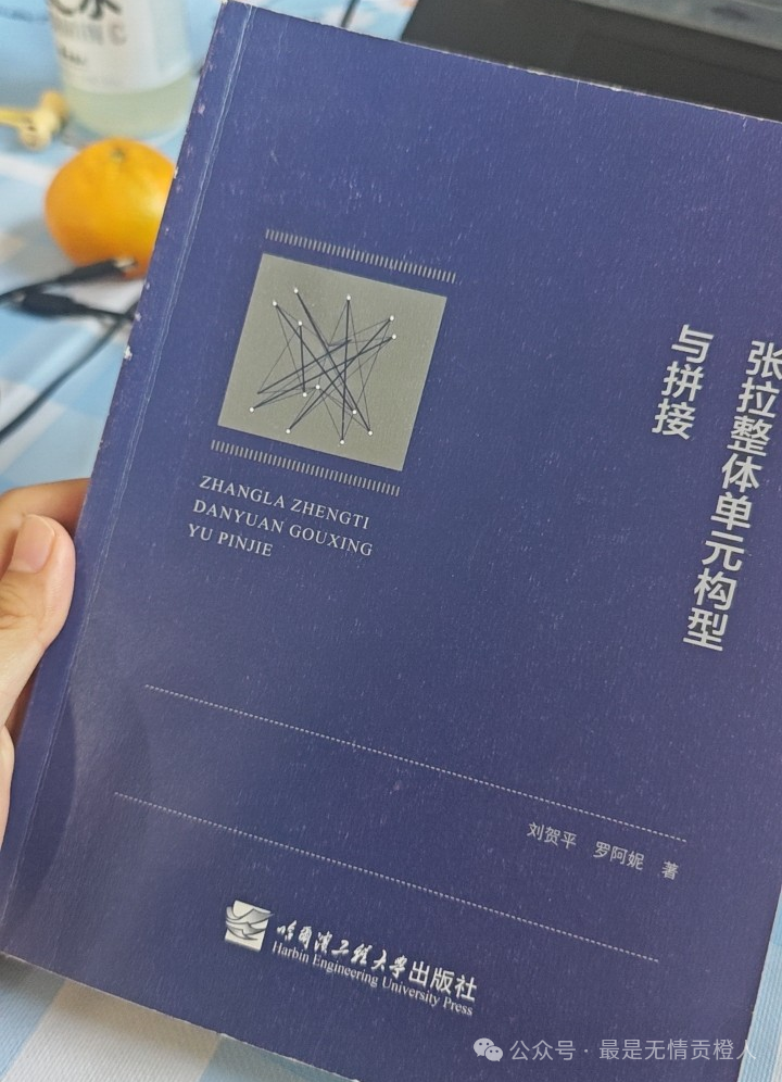
Code Source: Liu Heping, Luo Ani, “Tensile Integral Unit Configuration and Splicing” Chapters 2 and 3
(This book is very well written, logical, and engaging)
Utilizing the similarities between tensile structures and origami, replacing peaks with rods and valleys with cables, connects tensile structures with origami structures.
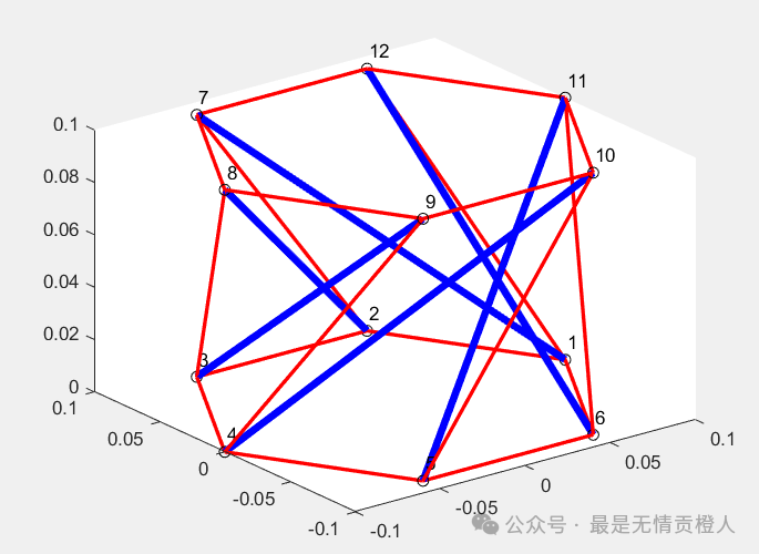
Taking MATLAB 2022 as an example, the code for drawing a single-layer Kresling is provided (based on this code, the surface can be completed; some papers do not complete the surface when studying performance).


% Initialize environment
clear all;
close all;
clc;
% ============================
% Input parameters
% ============================
p = 6; % Number of rods, representing the number of basic units of the structure
j = 1; % Configuration parameter, controlling the twisting relationship between the upper and lower circles
rd = 0.1; % Radius of the lower circle
ru = 0.1; % Radius of the upper circle
h = 0.1; % Height of the structure
% ============================
% Parameter calculations
% ============================
thet0 = 2 * pi / p; % Angle increment for each rod
ph0 = pi / 2 + j * pi / p; % Relative twisting angle
% ============================
% Node empty matrix
% ============================
N = [];
NU = []; % Lower circle node matrix
ND = []; % Upper circle node matrix
% Generate node coordinates
for idx = 0:p-1
% Lower circle nodes
nuix = rd * cos(idx * thet0); % Lower circle node x coordinate
nuiy = rd * sin(idx * thet0); % Lower circle node y coordinate
nui = [nuix; nuiy; 0]; % Lower circle node 3D coordinates
NU = [NU, nui];
% Upper circle nodes
ndix = ru * cos(ph0 + idx * thet0); % Upper circle node x coordinate
ndiy = ru * sin(ph0 + idx * thet0); % Upper circle node y coordinate
ndi = [ndix; ndiy; h]; % Upper circle node 3D coordinates
ND = [ND, ndi];
end
N = [NU, ND]; % Merge upper and lower circle node matrices to form a complete node matrix
% ============================
% Create connection matrix C
% ============================
% ============================
% Plotting
% ============================
figure;
plot3(N(1,:), N(2,:), N(3,:), ‘ko’); % Plot node distribution, black dots
for i = 1:size(N, 2)
text(N(1, i) + 0.005, N(2, i) + 0.005, N(3, i) + 0.005, num2str(i)); % Label node number
end
% ============================
% Rod connection matrix
% ============================
CBT = [-eye(p) eye(p)]; % Connection matrix, representing the connection relationship between rods and nodes
CB = CBT’; % Transpose matrix
B = N * CB; % Calculate rod vectors
% Draw rods
for i = 1:p
n1 = N(:, i); % Get the starting point of the rod
n2 = N(:, i) + B(:, i); % Get the endpoint of the rod
g_b = line([n1(1) n2(1)], [n1(2) n2(2)], [n1(3) n2(3)]); % Draw the connection line of the rod
set(g_b, ‘LineWidth’, 4, ‘color’, ‘b’); % Set rod line width and color (blue)
hold on;
end
% ============================
% Cable connection matrix
% ============================
CS = zeros(size(N, 1), size(N, 2)); % Initialize cable connection matrix
for i = 1:p
CS(:, i) = -1; % Connect lower circle nodes
CS(:, i + p) = 1; % Connect upper circle nodes
end
% ============================
% Cable matrix (e1 and e2)
% ============================
e1 = []; % Initialize cable matrix e1
e2 = []; % Initialize cable matrix e2
for i = 0:p-1
if i == 0
e1i = [-1 1 zeros(1, p-2)];
elseif i > 0 && i < p-1
e1i = [zeros(1, i) -1 1 zeros(1, p-i-2)];
else
e1i = [1 zeros(1, p-2) -1];
end
e1 = [e1; e1i]; % Append e1i to e1
end
% Create e2
CS00 = [zeros(p-j, j), eye(p-j); eye(j), zeros(j, p-j)];
e2 = CS00′;
% Form complete connection matrix CS1
CS1 = [e1 zeros(p, p); zeros(p, p) e1; -eye(p) e2];
CS = CS1;
CST = CS’; % Transpose matrix CST
% Cable matrix S
S = N * CST; % Cable matrix S is obtained by multiplying node matrix N with transpose matrix CST
% ============================
% Draw cables
% ============================
[nsr, nsc] = size(CST); % Get the number of rows and columns of CST
for i = 1:nsc
CSTi = CST(:, i); % Get each column of CST
n2n = find(CSTi == -1); % Find positions where CSTi has a value of -1
n1 = N(:, n2n); % Get coordinates of starting nodes
n2 = N(:, n2n) + S(:, i); % Get coordinates of ending nodes
% Draw cable segments
s_b = plot3([n1(1) n2(1)], [n1(2) n2(2)], [n1(3) n2(3)], ‘r’, ‘LineWidth’, 2); % Red cable
hold on;
end
% Ensure the figure is displayed after plotting is complete
hold off;
Running the above code will yield the following result:
This post has no commercial purpose and is solely for knowledge sharing. If there is any infringement, it will be deleted immediately.
Author’s note: Personal opinions are for reference only. I don’t remember what each line of code means as it has been a long time… I don’t check private messages often, so feel free to leave comments for discussion. I have a fragile heart, and I am not very skilled. I referenced AI, and this public account is mainly for recording life. I post whatever I want (I think this should be enough for stacking armor).