Numerical computation is an important tool in scientific research and engineering applications. When analytical solutions are difficult to obtain, MATLAB provides efficient methods for numerical differentiation and integration. This article starts from basic concepts and combines code examples to help beginners quickly master these two core skills.

1. Numerical Differentiation: Approximating Derivatives with Differences

1. Basic Principles

The core idea of numerical differentiation is to use the differences of function values to approximate derivatives.

Let the step size be , and expand the function and at the point using Taylor series, we can obtain:

From and , we can derive:

• Forward Difference:
• Backward Difference:
• Central Difference (higher accuracy):

2. MATLAB Implementation

Example: Calculate the derivative of on the interval :

clc; clear; close all;
h = pi/20; 
x0 = 0:h:pi;
y0 = sin(x0);
y1 = sin(x0+h);
y_1 = sin(x0-h);

yp = cos(x0);                       % Derivative values
df_for = (y1-y0)/h;                 % Forward difference
df_back =(y0-y_1)/h;                % Backward difference
df_center =(y1-y_1)/(2*h);          % Central difference
figure()
plot(x0,df_for,'r^')
hold on
plot(x0,df_back,'bs')
hold on
plot(x0,df_center,'yo')
hold on
plot(x0,yp,'k-')
legend('Forward Difference','Backward Difference','Central Difference','Derivative')
xlabel('$x$','interpreter','latex')
ylabel(['$rac{d 	ext{sin}(x)}{d x}$'],'interpreter','latex')

The results are shown in the figure below, which indicates a high agreement with the derivative function .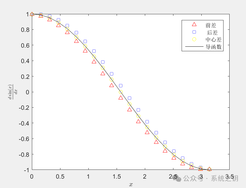

Numerical Integration: From Rectangular Method to Simpson’s Rule

1. Algorithm Principles

According to the definition of definite integrals:

Divide the integration interval into equal-width subintervals, with a step size of . The area of each subinterval is approximated using rectangles, yielding:

Left Rectangular Formula:

Right Rectangular Formula:

Taking the average of the two formulas gives:

Trapezoidal Formula:

Simpson’s Formula: Approximating the curve between every two adjacent subintervals with a parabola:

2. MATLAB Implementation

Example: Calculate (the theoretical value is .

• 2.1 Calculate integrals using the rectangular and trapezoidal formulas.

clc;clear all;close all;
n1 = 3;
n2 = 50;
for k =n1:n2
    h=pi/k;
    x = 0:h:pi; %length(x)=k+1
    f = sin(x); %length(f)=k+1
    I1(k) = sum(f(1:k))*h;  % Left rectangular formula
    I2(k) = sum(f(2:k+1))*h; % Right rectangular formula
    I3(k) = sum(f(2:k))*h+(f(1)+f(k+1))*h/2;  % Trapezoidal formula
end
figure()
kk = n1:n2;
plot(kk,I1(kk),'r^')
hold on
plot(kk,I2(kk),'bs')
hold on
plot(kk,I3(kk),'bo')
xlabel('Number of grids n')
ylabel('Integral value I')
legend('Left Rectangular Formula','Right Rectangular Formula','Trapezoidal Formula')

The results are shown below.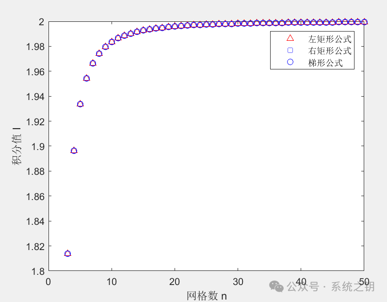

• 2.2 Calculate integrals using Simpson’s formula.

clc;clear all;close all;
n1 = 4;
n2 = 20;
for k =n1:2:n2
    h=pi/k;
    x = 0:h:pi; %length(x)=k+1
    f = sin(x); %length(f)=k+1
    I(k) = (f(1)+f(end))*h/3+sum(f(2:2:end-1))*4*h/3+sum(f(3:2:end-2))*2*h/3;
end
figure()
kk = n1:2:n2;
plot(kk,I(kk),'ro')
ylim([2.0,2.006])
xlabel('Number of grids n')
ylabel('Integral value I')
legend('Simpson’s Formula')

The results are shown in the figure below.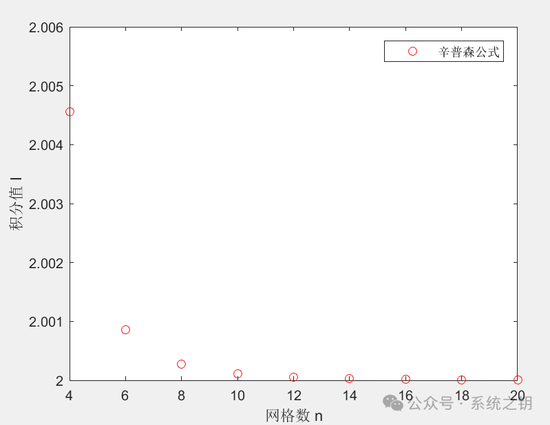

References

[1] Peng Fanglin, Fundamentals of Computational Physics (2nd Edition), Higher Education Press, 2024.8

ENDScan to Follow Us A complex world, simple rules