Data Analysis: Calculating and Plotting the Relationship Between Signal-to-Noise Ratio and Noise Intensity of the Double-Well Duffing Oscillator Based on Matlab

✅ Author Profile: A Matlab simulation developer passionate about research, skilled in data processing, modeling simulation, program design, obtaining complete code, reproducing papers, and scientific simulation.

🍎 Previous reviews can be found on my personal homepage:Matlab Research Studio

🍊 Personal motto: Investigate things to gain knowledge, complete Matlab code and simulation consultation available via private message.

Intelligent Optimization Algorithms Neural Network Prediction Radar Communication Wireless Sensors Power Systems

Signal Processing Image Processing Path Planning Cellular Automata Unmanned Aerial Vehicles

Physical Applications Machine Learning Series Workshop Scheduling Series Filtering and Tracking Series Data Analysis Series

Image Processing Series

🔥 Content Introduction

The Duffing oscillator, as a classic nonlinear dynamical system, has attracted significant attention due to its rich dynamical behaviors. In particular, the double-well Duffing oscillator exhibits unique stochastic resonance phenomena under external periodic driving and noise disturbances. Studying the relationship between the signal-to-noise ratio (SNR) and noise intensity of this oscillator not only aids in understanding the noise behavior of nonlinear systems but also provides a theoretical basis for applications such as signal detection and energy harvesting. This article will explain how to calculate and plot the relationship between the SNR and noise intensity of the double-well Duffing oscillator, involving model establishment, numerical simulation, data processing, and result analysis.

1. Double-Well Duffing Oscillator Model

The double-well Duffing oscillator can be described by the following second-order nonlinear ordinary differential equation:

x'' + δx' - αx + βx^3 = Acos(ωt) + ξ(t)

Where:

x represents the displacement of the oscillator;
x' and x'' represent velocity and acceleration, respectively;
δ is the damping coefficient, describing the energy dissipation of the system;
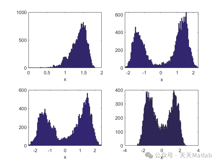
α and β are parameters related to the shape of the potential wells, determining the depth and width of the double wells. Typically, α > 0 and β > 0 ensure the existence of two stable equilibrium points, forming a double-well structure;
A and ω are the amplitude and frequency of the external periodic driving, respectively;
ξ(t) represents Gaussian white noise, with statistical properties given by:

<ξ(t)> = 0 (mean is zero)
<ξ(t)ξ(t')> = 2Dδ(t - t') (correlation function is the Dirac function), where D represents the noise intensity.

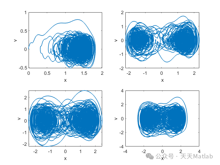
The above equation describes an oscillator affected by damping, nonlinear restoring force, periodic driving, and random noise. The double-well structure is key to the complex behaviors exhibited by this system, while noise introduces randomness, allowing the oscillator to transition between the two potential wells.

2. Numerical Simulation Method

Since the equation of the Duffing oscillator is nonlinear, it is usually difficult to obtain an analytical solution. Therefore, numerical simulation methods are required to solve this equation. Common numerical methods include:

Runge-Kutta Method: The Runge-Kutta method is a high-order single-step integration method characterized by high accuracy and good stability. The fourth-order Runge-Kutta method (RK4) is the most commonly used choice. This method approximates the true solution by estimating derivatives over multiple time steps.
Euler-Maruyama Method: A numerical method specifically designed for solving stochastic differential equations. It is the stochastic version of the Euler method, suitable for systems with additive noise.

To more accurately simulate the double-well Duffing oscillator, it is recommended to use the Runge-Kutta method in conjunction with methods for handling random noise. The specific implementation steps are as follows:

*   **Discretize Time:** Divide the time axis into discrete time steps `Δt`.  
*   **Convert to First-Order System:** Transform the second-order equation into two first-order equations:  
    ```  
    x' = v  
    v' = αx - βx^3 - δv + Acos(ωt) + ξ(t)  
    ```  
*   **Iterative Calculation:** Use the Runge-Kutta method to iteratively calculate the above first-order equations, obtaining the displacement `x(t)` and velocity `v(t)` at each time step.  
*   **Add Noise:** At each time step, generate a random number following a normal distribution with a mean of 0 and a standard deviation of `√(2DΔt)`, then add it as `ξ(t)` to the velocity update equation.

3. Calculation of Signal-to-Noise Ratio (SNR)

The signal-to-noise ratio is an indicator that measures the strength of the signal relative to the noise intensity. For the Duffing oscillator, it reflects the clarity of the periodic driving signal against the noise background. The steps to calculate SNR are as follows:

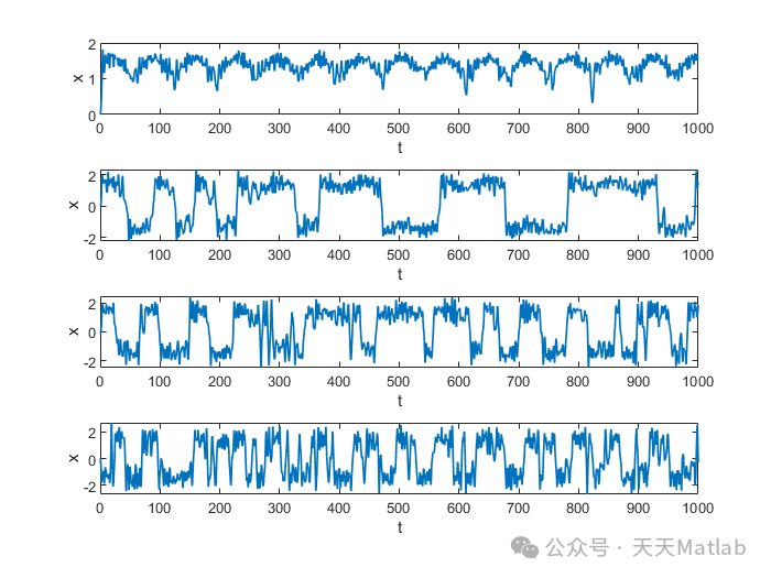
Time Domain Data Collection: Obtain the time series data of the oscillator’s displacement x(t) through numerical simulation. Ensure that the data is sufficiently long for subsequent spectral analysis. Typically, multiple cycles of the driving signal need to be simulated, discarding the initial transient process.
Spectral Analysis: Perform a Fourier transform (FFT) on the time domain data to obtain the frequency spectrum X(f). The frequency spectrum shows the energy distribution of the signal at different frequencies.
Determining Signal Power and Noise Power: In the frequency spectrum, find the peak corresponding to the driving frequency ω, which represents the signal power P_signal. Select a frequency range near the peak, excluding the influence of the signal peak, and calculate the average power within that frequency range as the noise power P_noise.
Calculate SNR: The signal-to-noise ratio can be calculated using the following formula:
```
SNR = 10log10(P_signal / P_noise)
```
The unit of SNR is decibels (dB).

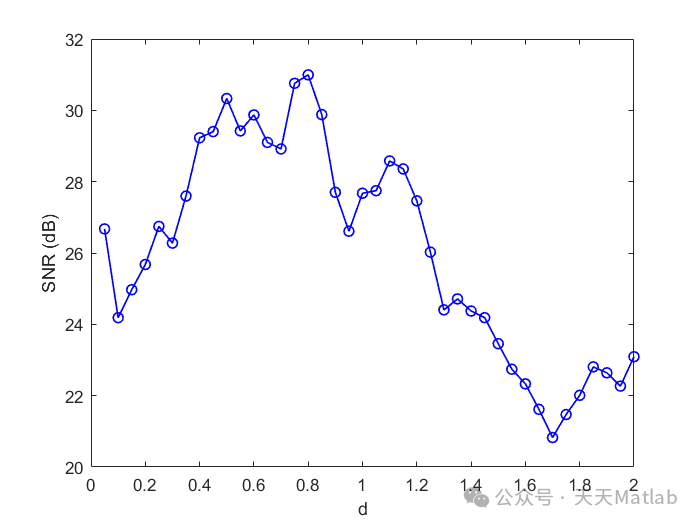
4. Plotting the Relationship Between SNR and Noise Intensity

To plot the relationship between SNR and noise intensity, the following steps need to be performed:

Loop Through Noise Intensities: Set a series of different noise intensity D values.
Numerical Simulation: For each noise intensity D value, perform numerical simulation to obtain the time series data of displacement x(t).
Calculate SNR: Calculate the SNR value corresponding to each noise intensity using the aforementioned method.
Plot the Relationship Graph: Plot a scatter plot or curve graph with noise intensity D on the x-axis and SNR on the y-axis.

5. Result Analysis and Discussion

After plotting the relationship graph between SNR and noise intensity, the results can be analyzed and discussed. Typically, the following phenomena are observed:

Stochastic Resonance: At lower noise intensities, SNR increases with the increase of noise intensity, reaching a peak. This indicates that moderate noise can enhance the strength of the signal, which is the phenomenon of stochastic resonance. Noise facilitates the transition of the oscillator between the two potential wells, thereby responding better to the periodic driving signal.
Over-Noise Suppression: When the noise intensity exceeds a certain threshold, SNR decreases with the increase of noise intensity. This is because excessive noise can drown out the signal, making it difficult to detect effectively.
Parameter Influence: The parameters of the Duffing oscillator (e.g., damping coefficient δ, double-well shape parameters α and β, and the amplitude A and frequency ω of the driving signal) significantly affect the relationship between SNR and noise intensity. For example, a larger damping will weaken the system’s response to noise, thereby affecting the strength of stochastic resonance.

⛳️ Running Results

🔗 References

[1] Zhang Mei, Luo Shiyu, Shao Mingzhu. Channel Effect and Optical Bistability Effect of Superlattice Quantum Wells [J]. Semiconductor Optoelectronics, 2008, 29(3):4. DOI:CNKI:SUN:BDTG.0.2008-03-012.

[2] Cao Baofeng, Li Peng, Li Xiaoqiang, et al. Weak Pulse Signal Detection and Parameter Estimation Based on Strongly Coupled Duffing Oscillator [J]. Acta Physica Sinica, 2019(8):11. DOI:10.7498/aps.68.20181856.

📣 Partial Code

🎈 Some theoretical references are from online literature; please contact the author for removal if there is any infringement.

👇 Follow me to receive a wealth of Matlab e-books and mathematical modeling materials.

🏆 Our team specializes in guiding customized MATLAB simulations in various research fields to support your research dreams:

🌈 Various intelligent optimization algorithm improvements and applications

Production scheduling, economic scheduling, assembly line scheduling, charging optimization, workshop scheduling, departure optimization, reservoir scheduling, three-dimensional packing, logistics site selection, cargo location optimization, bus scheduling optimization, charging pile layout optimization, workshop layout optimization, container ship loading optimization, pump combination optimization, medical resource allocation optimization, facility layout optimization, visual domain base station and drone site selection optimization, knapsack problem, wind farm layout, time slot allocation optimization, optimal distribution of distributed generation units, multi-stage pipeline maintenance, factory-center-demand point three-level site selection problem, emergency material distribution center site selection, base station site selection, road lamp post arrangement, hub node deployment, transmission line typhoon monitoring devices, container scheduling, unit optimization, investment optimization portfolio, cloud server combination optimization, antenna linear array distribution optimization, CVRP problem, VRPPD problem, multi-center VRP problem, multi-layer network VRP problem, multi-center multi-vehicle VRP problem, dynamic VRP problem, two-layer vehicle routing planning (2E-VRP), electric vehicle routing planning (EVRP), hybrid vehicle routing planning, mixed flow workshop problem, order splitting scheduling problem, bus scheduling optimization problem, flight shuttle vehicle scheduling problem, site selection path planning problem, port scheduling, port bridge scheduling, parking space allocation, airport flight scheduling, leak source localization.

🌈 Machine learning and deep learning time series, regression, classification, clustering, and dimensionality reduction

2.1 BP time series, regression prediction, and classification

2.2 ENS voice neural network time series, regression prediction, and classification

2.3 SVM/CNN-SVM/LSSVM/RVM support vector machine series time series, regression prediction, and classification

2.4 CNN|TCN|GCN convolutional neural network series time series, regression prediction, and classification

2.5 ELM/KELM/RELM/DELM extreme learning machine series time series, regression prediction, and classification

2.6 GRU/Bi-GRU/CNN-GRU/CNN-BiGRU gated neural network time series, regression prediction, and classification

2.7 Elman recurrent neural network time series, regression prediction, and classification

2.8 LSTM/BiLSTM/CNN-LSTM/CNN-BiLSTM long short-term memory neural network series time series, regression prediction, and classification

2.9 RBF radial basis neural network time series, regression prediction, and classification

2.10 DBN deep belief network time series, regression prediction, and classification

2.11 FNN fuzzy neural network time series, regression prediction

2.12 RF random forest time series, regression prediction, and classification

2.13 BLS broad learning time series, regression prediction, and classification

2.14 PNN pulse neural network classification

2.15 Fuzzy wavelet neural network prediction and classification

2.16 Time series, regression prediction, and classification

2.17 Time series, regression prediction, and classification

2.18 XGBOOST ensemble learning time series, regression prediction, and classification

2.19 Transform various combinations of time series, regression prediction, and classification

Directions cover wind power prediction, photovoltaic prediction, battery life prediction, radiation source identification, traffic flow prediction, load prediction, stock price prediction, PM2.5 concentration prediction, battery health status prediction, electricity consumption prediction, water body optical parameter inversion, NLOS signal recognition, precise prediction of subway stops, transformer fault diagnosis.

🌈 In the field of image processing

Image recognition, image segmentation, image detection, image hiding, image registration, image stitching, image fusion, image enhancement, image compressed sensing.

🌈 In the field of path planning

Traveling salesman problem (TSP), vehicle routing problem (VRP, MVRP, CVRP, VRPTW, etc.), UAV three-dimensional path planning, UAV collaboration, UAV formation, robot path planning, grid map path planning, multimodal transport problems, electric vehicle routing planning (EVRP), two-layer vehicle routing planning (2E-VRP), hybrid vehicle routing planning, ship trajectory planning, full path planning, warehouse patrol.

🌈 In the field of UAV applications

UAV path planning, UAV control, UAV formation, UAV collaboration, UAV task allocation, UAV secure communication trajectory online optimization, vehicle collaborative UAV path planning.

🌈 In the field of communication

Sensor deployment optimization, communication protocol optimization, routing optimization, target localization optimization, Dv-Hop localization optimization, Leach protocol optimization, WSN coverage optimization, multicast optimization, RSSI localization optimization, underwater communication, communication upload and download allocation.

🌈 In the field of signal processing

Signal recognition, signal encryption, signal denoising, signal enhancement, radar signal processing, signal watermark embedding and extraction, electromyography signals, electroencephalography signals, signal timing optimization, electrocardiogram signals, DOA estimation, encoding and decoding, variational mode decomposition, pipeline leakage, filters, digital signal processing + transmission + analysis + denoising, digital signal modulation, bit error rate, signal estimation, DTMF, signal detection.

🌈 In the field of power systems

Microgrid optimization, reactive power optimization, distribution network reconstruction, energy storage configuration, orderly charging, MPPT optimization, household electricity.

🌈 In the field of cellular automata

Traffic flow, crowd evacuation, virus spread, crystal growth, metal corrosion.

🌈 In the field of radar

Kalman filter tracking, trajectory association, trajectory fusion, SOC estimation, array optimization, NLOS recognition.

🌈 Workshop scheduling

Zero-wait flow shop scheduling problem (NWFSP) , permutation flow shop scheduling problem (PFSP) , hybrid flow shop scheduling problem (HFSP) , zero idle flow shop scheduling problem (NIFSP), distributed permutation flow shop scheduling problem (DPFSP), blocking flow shop scheduling problem (BFSP).

👇