Article Overview
Flat Field Correction (FFC) is a common technique in image processing used to eliminate uneven illumination or sensor response non-uniformity in images. FFC typically requires a flat field image, which is captured under uniform lighting conditions, to correct the target image.
The following is a simplified FFC program based on MATLAB, designed to read RAW format images with a resolution of 7680×4320, selecting a 4×4 pixel area as one block, with each block sharing one correction coefficient for flat field correction. The corrected image will be saved as a new RAW file.
The significance of the simplified flat field correction program lies in its ability to reduce storage resource usage significantly when certain embedded systems lack sufficient storage resources to perform full flat field correction on high-resolution images.
Algorithm Principle
The principle of flat field correction
The goal of flat field correction is to eliminate uneven illumination or sensor response non-uniformity in images. Its basic principles are as follows:
1. Flat Field Image: The flat field image is captured under uniform lighting conditions, reflecting the sensor’s uneven response and the uneven distribution of illumination.
2. Correction Formula: The correction formula is as follows:

Where, Itarget is the target image, flat_data is the flat field image, and flat_mean is the average value of the flat field image.
3. Correction Effect: After correction, the non-uniformity in the target image is eliminated, and the image quality is improved.
Improvements:
1. Block Processing Optimization:
The image is divided into 4×4 pixel blocks;
Each block shares one correction coefficient (block mean/global mean).
2. Boundary Processing:
Added image size checks to ensure divisibility by block size;
Used the min function to handle boundary blocks.
3. Computational Efficiency:
Explicit loops are used to process each block for better understanding.
5. Correction Formula:
Correction Coefficient = Global Mean of Flat Field Image / Current Block Mean;
Target Pixel Value = Original Value × Correction Coefficient.
Program Architecture
Code Description:
1. Input and Output:
◦ Input includes the target image file (input_file) and the flat field image file (flat_file), both in RAW format with a resolution of 7680×4320 and a bit depth of 16 bits. (Effective bit depth is 12 bits, with a saturation value of 4095).
◦ Output is the corrected RAW file (output_file), saved as 16 bits.
2. Flat Field Correction Logic:
◦ Read the target image and flat field image, extracting the lower 12 bits of effective data.
◦ Divide the flat field image into blocks of 4×4 pixels, calculating the mean for each block.
◦ Calculate the average value of the flat field image (flat_mean).
◦ Each block mean divided by the overall image mean gives the correction coefficient, calculated using the formula:

◦ Multiply the correction coefficient by the pixel values of that block to obtain the corrected image, using the formula:

◦ Limit the corrected data to the effective range of 12 bits (0~4095).
◦ Store the corrected data as 16 bits (high bits padded with 0) and save it as a RAW file.
3. Data Recovery:
◦ The corrected data needs to be restored to 16 bits to meet the storage format of RAW files.
Code Implementation
The MATLAB code implementation is as follows:
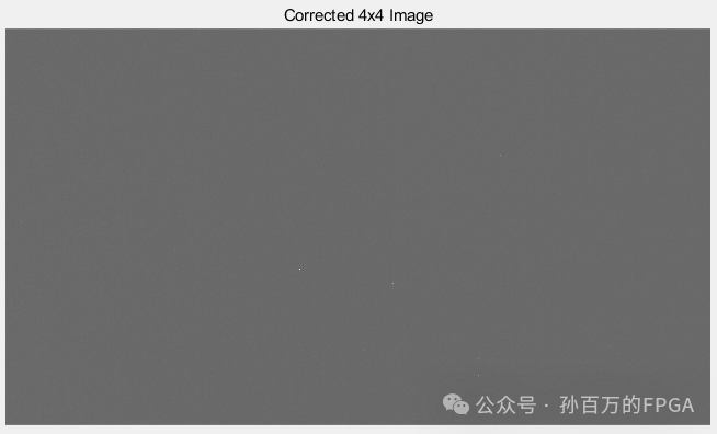
clc;clear;tic;% Image flat field correction module Simplified correction algorithmflat_field_correction_4x4_block('Image0_8K.raw', 'Image0_8K.raw', 'Image0_8K_corrected_4x4s.raw');function flat_field_correction_4x4_block(input_file, flat_file, output_file) % Parameter description: % input_file : Path to the input RAW format target image file % flat_file : Path to the input RAW format flat field image file % output_file: Path to the output corrected RAW file % Image parameters width = 7680; % Image width height = 4320; % Image height bit_depth = 16; % Image bit depth block_size = 4; % Group size (4x4) % Check if image dimensions are divisible by block size if mod(width, block_size) ~= 0 || mod(height, block_size) ~= 0 error('Image dimensions must be divisible by block size'); end % Read target image fid = fopen(input_file, 'rb'); if fid == -1 error('Cannot open target image file'); end target_data = fread(fid, [width, height], 'uint16'); raw_data_s = transpose(target_data); figure;subplot(1,2,1);imshow(raw_data_s,[0,4096]);title('Original Image'); fclose(fid); % Read flat field image fid = fopen(flat_file, 'rb'); if fid == -1 error('Cannot open flat field image file'); end flat_data = fread(fid, [width, height], 'uint16'); fclose(fid); % Convert to double precision target_data = double(target_data); flat_data = double(flat_data); % Calculate global mean of flat field image flat_global_mean = mean(flat_data(:)); % Initialize corrected image corrected_data = zeros(size(target_data)); % Calculate correction coefficient for each block and apply for row = 1:block_size:height for col = 1:block_size:width % Get current 4x4 block row_end = min(row+block_size-1, height); col_end = min(col+block_size-1, width); % Extract flat field image block flat_block = flat_data(col:col_end, row:row_end); % Calculate block mean block_mean = mean(flat_block(:)); % Calculate correction coefficient correction_factor = flat_global_mean / block_mean; % Extract target image block and apply correction target_block = target_data(col:col_end, row:row_end); corrected_block = target_block * correction_factor; % Store corrected block corrected_data(col:col_end, row:row_end) = corrected_block; end end % Limit data range and convert back to 16bit corrected_data = max(min(corrected_data, 4095), 0); corrected_data_s = transpose(corrected_data); subplot(1,2,2);imshow(corrected_data_s,[0,4096]);title('Corrected 4x4 Image'); % Save corrected image fid = fopen(output_file, 'wb'); if fid == -1 error('Cannot create output file'); end fwrite(fid, corrected_data, 'uint16'); fclose(fid); disp(['Flat field correction completed! Corrected image saved to: ' output_file]);endExample of image processing before and after output:

It can be seen that there is a significant vignetting on the left side of the original image compared to the right side. The corrected image shows overall uniformity, but some noise and bad pixels remain unprocessed.
General flat field correction can be fully successful, but simplified flat field correction still has some flaws.
Simplified Flat Field Correction
General Flat Field Correction

Notes
1. Requirements for Flat Field Image:
◦ The flat field image should be captured under uniform lighting conditions and should match the shooting conditions of the target image.
◦ The flat field image should avoid containing any target objects or noise.
2. Data Range Limitation:
◦ The corrected data needs to be limited to the effective range of 12 bits (0~4095) to avoid data overflow.
3. Performance Optimization:
◦ For high-resolution images of 7680×4320, the program may take a long time to run. Consider using MATLAB’s parallel computing features (such as parfor) to optimize performance.
4. File Path:
◦ Ensure that the input and output file paths are correct to avoid file read/write errors.