Click the blue text above to follow us!
Author: Daniel
Date: 2020/8/25
Problem-oriented, starting from scratch, quickly getting started, learning efficiently, and mastering Matlab programming.
Hello everyone! Previously, we released two articles on Matlab two-dimensional plotting:
.Matlab Introduction Tutorial | 008 Two-Dimensional Plotting: A Comprehensive Guide to the plot Function
.Matlab Introduction Tutorial | 009 Two-Dimensional Plotting: After reading this article, you will be able to plot all elementary functions!
Have you practiced the methods mentioned in those articles? Have you mastered them? Today, we will discuss the usage of other plotting functions and teach you a universal formula that will help you grasp the essentials of all plotting functions.
Before we start, let me tell you a joke:
At the last class reunion, they said they wanted to play Mahjong, but I didn’t know how. So a top student told me an amazing formula:
And I won, where it could equal 0. Wow! I learned Mahjong in just one minute!
The deeper meaning of this joke is:How to express complex ideas clearly and effectively—using mathematical language!
Back to the topic! There are many Matlab plotting functions, for example: univariate function plotting functions include:<span>plot, fplot, polarplot</span>, statistical plotting functions include:<span>bar, pie</span>, and spatial curve and surface plotting functions include:<span>plot3, mesh, surf</span>, etc. If we learn each one individually and discuss them one by one, it will take a lot of time, much more complex than playing Mahjong!
Today, I will tell you a universal plotting formula and steps that will allow you to grasp the essentials of Matlab plotting in just one minute!
Main Points of This Article
- Universal Plotting Formula
- Universal Plotting Steps
<span>fplot, polarplot, mesh</span>Examples
Universal Plotting Formula
Universal Plotting Formula:
<span>plotname(X,Y,Z,PropertyName,PropertyValue)</span>
Translated into English as:
<span>Plot Function Name (X, Y, Z, Property Name, Property Value)</span>
For two-dimensional plotting, drop one variable<span>Z</span>. The<span>plotname</span> can be any of the plotting functions listed above:<span>plot, fplot, bar, mesh,...</span>
Let’s take a simple example:
x = linspace(0,2*pi,100)
y = sin(x)

plot(x,y,'linewidth',1.5,'color','m')
The meaning of the third line is that the plotted image has a line width of 1.5pt and the line color is magenta. Here, “Property Name” and “Property Value” always appear in pairs.
Universal Plotting Steps
DPML Plotting Method:
- D (Define): Define the independent variable array and function array;
- P (Plot): Draw the graph;
- M (Mark): Make marks;
- L (Label): Set labels.
Application Examples
<span>plot, fplot</span> functions are the foundation of all other plotting functions; once you master the usage of<span>plot</span>, you can easily understand the other plotting functions!
Example 1. Plotting the sine function on the graph.
% Eg001
% sinx
% 4 cycles=================================================================================
clf

fplot(@(x) sin(x),[-6*pi,6*pi],'linewidth',2.5,'color','m')%  define, plot

set(gca,'Xtick',[-4*pi,-3*pi,-2*pi,-pi,0,pi,2*pi,3*pi,4*pi],'Ytick',[-1,-0.5,0,0.5,10])% label
set(gca,'XtickLabel',{'-4\pi';'-3\pi';'-2\pi';'-\pi';'0';'\pi';'2\pi';'3\pi';'4\pi'})
set(gca,'YtickLabel',{'-1';'-0.5';'0';'0.5';'1'})

hold on

plot([-6*pi 6*pi],[0 0],':r')% plot

axis equal
box off
grid on

title('\fontsize{14}\it y = sin x')% label
xlabel('\fontsize{14}\it x')
ylabel('\fontsize{14}\it y')
Code Explanation:
-
<span>clf</span>clears the previous image in the graphics window. -
Here, we use the
<span>fplot</span>function, which has two differences from<span>plot</span>: (1)<span>plot</span>requires manually setting the range of the independent variable array and step size, while<span>fplot</span>automatically sets them and can set different densities of points according to the function’s changing trend. (2)<span>fplot</span>combines the first two steps of the universal plotting method: define and plot:<span>fplot(@(x) sin(x))</span>,<span>@(x)</span>defines the independent variable, and the function expression defines the function. Note that operators in the function expression should use array operators. -
<span>[-6*pi,6*pi]</span>indicates the domain,<span>'linewidth',2.5,'color','m'</span><code><span> is as explained before, emphasizing that strings should be enclosed in single quotes.</span> -
Next, the three
<span>set</span>commands are easy to understand: manually set which points to mark on the axis, label the short vertical ticks on the axis, and label the short horizontal ticks on the axis.<span>gca</span>is probably an abbreviation for get current axes, referring to creating or accessing the current coordinate system of the graph. Sometimes, a single graph window may have multiple subplots, which may involve multiple coordinate systems, and using<span>gca</span>indicates the current coordinate system. -
<span>hold on</span>overlays a new graph on the existing graph in the same coordinate system. -
<span>plot([-6*pi 6*pi],[0 0],':r')</span><span>, here </span><code><span>x=[-6*pi 6*pi],y=[0 0]</span>, tells the independent variable and function arrays, with numbers separated by spaces. Since there are only two points, it draws a horizontal line,<span>':r'</span>indicates that the line style is dashed and the color is red. -
<span>axis equal</span>,<span>box off</span>, and<span>grid on</span>: a set of functions for beautifying the graph; the first sets the unit length of the x and y axes to be equal; the second turns off the top and right borders of the graph frame; the third turns on the grid lines. -
<span>title</span>,<span>xlabel</span>, and<span>ylabel</span>:<span>title</span>adds a title to the graph, centered above the graph frame;<span>xlabel,ylabel</span>set the names of the axes. Note that strings should be enclosed in single quotes.
The resulting image is:

Example 2. Plotting a polar coordinate equation:
% Eg002
% Polar Coordinate Equation

clf
% Define independent variable and function array (D)
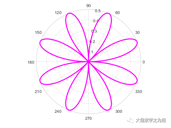
theta = 0:0.01:2*pi;
rho = sin(2*theta).*cos(2*theta);

% Plotting (P)
polarplot(theta,rho,'linewidth',1,'color','r')

% Label (L)
title('\fontsize{14}\it r = sin 2\theta cos 2\theta')
Code Explanation:
- This uses the three steps: D, P, L.
- The polar coordinate plotting function is
<span>polarplot</span>.
The resulting image is:
Example 3. Plotting a surface mesh:
% Eg003
% Example of mesh usage

% Define independent variable and function array (D)
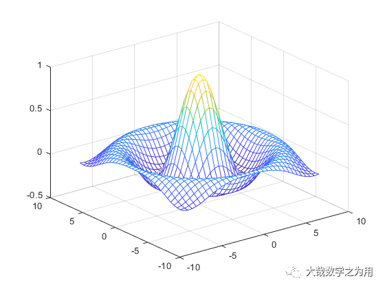
[X,Y] = meshgrid(-8:.5:8);
R = sqrt(X.^2 + Y.^2) + eps;
Z = sin(R)./R;

% Plotting (P)
mesh(X,Y,Z)

% Label (L)
title('Z = \frac{sin(\sqrt{x^2+y^2})}{\sqrt{x^2+y^2}}')
Code Explanation:
- This uses the three steps: D, P, L.
- The three-dimensional plotting function
<span>mesh</span>and<span>surf</span>differ in that:<span>mesh</span>displays the surface with colored gradient mesh lines, with color changing according to the height (i.e., the value) of the points on the surface, while<span>surf</span>displays the surface with color gradients in connected flat blocks.
The resulting image is:
Summary
Today we learned a universal plotting formula, a universal plotting step (DPML), several plotting functions, and some parameters and commands for controlling image properties. By grasping these two points and applying them flexibly, you can quickly master various Matlab plotting techniques. Finally, here are some suggestions:
- Some steps can be combined, and some steps can be omitted, apply flexibly according to actual needs;
- Be proactive in seeking help: In the command window, type:
<span>lookfor keyword</span>or<span>help keyword</span>to search for related topics.

Long press to identify the QR code and reply:003, to receive videos and e-books
Long press the QR code above and reply:003, to receive 2.5G of Matlab videos and introductory advanced e-books!
References
[1] Charles F. Van Loan, K. V. Daisy Fan, Insight Through Computing.
[2] Zhang Zhiyong, Mastering MATLAB R2011A.
Previous Recommendations .Matlab Introduction Tutorial | 009 Two-Dimensional Plotting: After reading this article, you will be able to plot all elementary functions! .Matlab Introduction Tutorial | 008 Two-Dimensional Plotting: A Comprehensive Guide to the plot Function。Matlab Introduction Tutorial | 007 Programming Example (Part 2): Calculating the Approximate Value of Pi。Matlab Introduction Tutorial | 007 Programming Example (Part 1): Calculating the Approximate Value of Pi。Matlab Introduction Tutorial | 006 Programming Example: Calculating the Approximate Value of e 。Matlab Introduction Tutorial | 005 Programming Example: Finding the Extremes of a Quadratic Function on a Closed Interval。Matlab Introduction Tutorial | 004 Programming Example: The Problem of Earth’s Surface Area Growth。MATLAB Introduction Tutorial | 003 Basic Knowledge。Matlab Advanced Tutorial | Extracting Brightness from Black and White Photos to Create Color Maps。Matlab Introduction Tutorial | 002 Long-term Investment Compound Interest Problem。Matlab Introduction Tutorial | 001 The Volume of a Sphere Problem。Installation Tutorial | MATLAB 2016b~2018b Installation Tutorial

Welcome to “Like,” “See Again,” and Leave a Message! Your support is our motivation to continue!