
Ordinary differential equations are mathematical models we frequently encounter when solving practical problems. When specifically solving ordinary differential equations, certain boundary conditions must be added. There are typically two types of boundary conditions: initial conditions and boundary conditions. The boundary value problem corresponding to boundary conditions is called the boundary value problem. This article provides a brief introduction to the shooting method for solving two-point boundary value problems.
For equations commonly found in engineering:
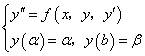
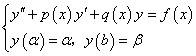
When f is linear with respect to y and y’, the above expression represents a linear two-point boundary value problem, which can be expressed as:
The basic principle of the shooting method is to transform the two-point boundary value problem into the following form of an initial value problem:
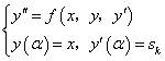
Here, sk is the slope of y at a. Let z=y’, the above second-order equation can be reduced to a first-order system of equations:
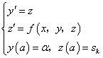
Thus, the boundary value problem becomes finding an appropriate sk such that the solution of the initial value problem for the above system of equations satisfies the original boundary value problem’s right boundary condition y(b)=β, thereby obtaining the solution to the boundary value problem. In this way, the numerical solution of a two-point boundary value problem is transformed into the numerical solution of a first-order system of equations’ initial value problem. All numerical methods for initial value problems can be applied here. The key issue is how to find an appropriate initial slope trial value sk.
For a given sk, let the solution of the initial value problem be y(x,sk), which is an implicit function of sk. Assuming y(x,sk) varies continuously with sk, we denote it as y(b,s)-β=0, thus the sk we are looking for is the root of the equation. The root of the above equation can be found using iterative methods. For example, using the secant method:


Thus, a simple computational process can be followed to find the solution. First, two initial slopes s0 and s1 are given as initial conditions for the initial value problem. Using the numerical methods for the first-order system of equations, we obtain the function values at the right endpoint of the interval: y(b,s0) and y(b,s1). If:
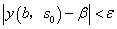
or
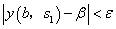
then use y(b,s0) or y(b,s1) as the solution to the two-point boundary value problem. Otherwise, use the secant method to find s2, similarly obtaining y(b,s2) and checking if it meets the accuracy requirements.
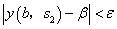
Repeat this until some sk satisfies:
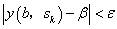
The resulting y(xi) and y’i=z(xi) are the function values and their first derivative values of the boundary value problem. The above equation resembles shooting a target, with sk acting as the bullet’s launch slope, and y(b) as the target, hence the name shooting method.
It is worth noting that for linear boundary value problems, a simple and practical method is to use analytical thinking to transform it into two initial value problems:
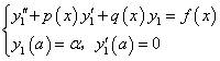
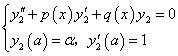
Finding the solutions y1(x) and y2(x) for these two initial value problems, if y2(b)≠0, it can be easily verified that the solution to the linear two-point boundary value problem is:
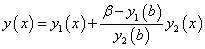
The following is a Matlab program shared by Sina blog author xianfa110 for solving two-point boundary value problems using the shooting method, for reference only.
function varargout = shooting_two_point_boundary(varargin)
% =====================
% Function name: shooting_two_point_boundary.m
% Based on shooting method to compute two-point boundary value problem
% Only for second-order differential equations
% author: xianfa110.
% blog.sina.com.cn/xianfa110
% Function form:
% [result,err,z0] = shooting_two_point_boundary(@fun,[y_0,y_end],[x_0,x_1],h);
% Input:
% fun = function name;
% y_0 = initial value of the function;
% y_end = final value of the function;
% x_0 = initial value of the independent variable;
% x_end = final value of the independent variable;
% h = integration step size;
% Output:
% result = [x,y];
% err = error;
% z0 = initial value of y’;
% =====================
% Function fun: 4y”+yy’ = 2x^3 +16 ; 2<= x <=3
% Implementation:
% function f = fun(y,x)
% dy = y(2);
% dz = (2*x^3+16-y(1)*y(2))/4;
% f = [dy,dz];
% =====================
% Note: y(1) = y, y(2) = y’.
% =====================
F = varargin{1};
y_0 = varargin{2}(1);
y_end = varargin{2}(2);
x_0 = varargin{3}(1);
x_1 = varargin{3}(2);
ts = varargin{4};
t0 = x_0-0.5;
flg = 0;
kesi = 1e-6;
y0 = rkkt(F,[y_0,t0],x_0,x_1,ts);
n = length(y0(:,1));
if abs(y0(n,1)-y_end)<=kesi
flg=1;
else
t1=t0+1;
y1=rkkt(F,[y_0,t1],x_0,x_1,ts);
if abs(y1(n,1)-y_end)<=kesi
flg=1;
end
end
if flg ~= 1
while abs(y1(n,1)-y_end) > kesi
% ==Interpolation method to solve nonlinear equation==
t2 = t1-(y1(n,1)-y_end)*(t1-t0)/(y1(n,1)-y0(n,1));
y2 = rkkt(F,[y_0,t2],x_0,x_1,ts);
t0=t1;
t1=t2;
y0=y1;
y1=y2;
end
end
x = x_0:ts:x_1;
out = [x’,y1(:,1)];
varargout{1} = out;
varargout{2} = abs(y1(n,1)-y_end);
varargout{3} = t1;

This article is compiled based on online materials.

Disclaimer: This WeChat article is reposted for non-commercial educational and research purposes and does not imply support for its views or confirm the authenticity of its content. The copyright belongs to the original author. If there are copyright issues with the reprinted material, please contact us immediately, and we will change or delete the relevant articles to protect your rights!