Implement PCA/TSNE/KPCA/LDA/SVD dimensionality reduction algorithms (Python code). The information available online on various dimensionality reduction algorithms is inconsistent, and most do not provide source code. Here is a GitHub project that organizes 11 classic data extraction (dimensionality reduction) algorithms implemented in Python, including: PCA, LDA, MDS, LLE, TSNE, etc., along with related materials and demonstration effects;It is verysuitable for beginners in machine learning and those just starting in data mining.

01 Why Perform Dimensionality Reduction?
Dimensionality reduction refers to using a set of vectors with a count of d, Zi, to represent the useful information contained in a set of vectors with a count of D, Xi, where d<D; in simple terms, it means reducing high-dimensional data to low dimensions.
Typically, we find that most datasets have dimensions reaching hundreds or even thousands, while the classic MNIST dataset has dimensions of 64.
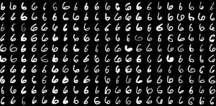
MNIST handwritten digit dataset
However, in practical applications, the useful information we need does not require such high dimensions, and the number of samples required increases exponentially with each additional dimension, which can lead to a significant “curse of dimensionality”; dimensionality reduction can achieve:
-
Making the dataset easier to use
-
Ensuring that variables are independent of each other
-
Reducing algorithm computational costs
-
Removing noise
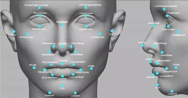
Once we can correctly handle this information and perform dimensionality reduction effectively, it will greatly help reduce computational load, thus improving machine efficiency. Dimensionality reduction is also commonly applied in areas such as text processing, facial recognition, image recognition, and natural language processing.
02 Principles of Dimensionality Reduction
High-dimensional data often appears sparse, so during the dimensionality reduction process, we usually reduce some data, including redundant data, invalid information, and repeated expressions.
For example: if we have a 1024*1024 image, where all positions except the central 50*50 area are zero, this zero information can be classified as useless information; for symmetric shapes, the information in the symmetric parts can be classified as repeated information.

Therefore, most classic dimensionality reduction techniques are based on this principle, which can be divided into linear and nonlinear dimensionality reduction methods, with nonlinear dimensionality reduction further divided into kernel-based and eigenvalue-based methods.
-
Linear Dimensionality Reduction Methods:
PCA, ICA, LDA, LFA, LPP (linear representation of LE)
-
Nonlinear Dimensionality Reduction Methods:
Kernel-based nonlinear dimensionality reduction methods—KPCA, KICA, KDA
Eigenvalue-based nonlinear dimensionality reduction methods (manifold learning)—ISOMAP, LLE, LE, LPP, LTSA, MVU
Heucoder, a master’s student in computer technology at Harbin Institute of Technology, has organized 12 classic dimensionality reduction algorithms including PCA, KPCA, LDA, MDS, ISOMAP, LLE, TSNE, AutoEncoder, FastICA, SVD, LE, LPP, and provided related materials, codes, and demonstrations. Below, we will mainly introduce the specific operation of the dimensionality reduction algorithm using the PCA algorithm as an example.
03 Principal Component Analysis (PCA) Dimensionality Reduction Algorithm
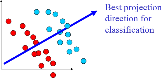
PCA is a mapping method that projects from high-dimensional space to low-dimensional space, and it is the most basic unsupervised dimensionality reduction algorithm. Its goal is to project in the direction of maximum data variance, or in the direction that minimizes reconstruction error. It was proposed by Karl Pearson in 1901 and belongs to linear dimensionality reduction methods. The principles related to PCA are usually referred to as maximum variance theory or minimum error theory. These two have consistent goals, but different focuses in the process.
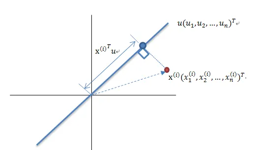
Maximum Variance Theory Dimensionality Reduction Principle
To reduce a set of N-dimensional vectors to K dimensions (K greater than 0 and less than N), the goal is to select K unit orthogonal bases, such that the covariance COV(X,Y) between each field is 0, while the variance of the fields is as large as possible. Therefore, maximum variance maximizes the variance of the projected data. In this process, we need to find the optimal projection space Wnxk of the dataset Xmxn, covariance matrix, etc. The algorithm flow is as follows:
-
Algorithm Input: Dataset Xmxn;
-
Calculate the mean Xmean of the dataset X by column, then let Xnew=X−Xmean;
-
Calculate the covariance matrix of Xnew, denoted as Cov;
-
Calculate the eigenvalues and corresponding eigenvectors of the covariance matrix Cov;
-
Sort the eigenvalues from largest to smallest, select the largest k, and then form the eigenvector matrix Wnxk from the corresponding k eigenvectors as column vectors;
-
Calculate XnewW, which projects the dataset Xnew onto the selected eigenvectors, yielding the reduced dataset XnewW we need.
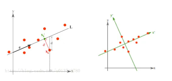
Minimum Error Theory Dimensionality Reduction Principle
Minimum error aims to minimize the average projection cost in linear projection, during which we need to find parameters such as the squared error evaluation function J0(x0).
For detailed steps, please refer to “Implementing Principal Component Analysis (PCA) Algorithm from Scratch”:
https://blog.csdn.net/u013719780/article/details/78352262
04 PCA Code Implementation
The code for the PCA algorithm is as follows:
from __future__ import print_function
from sklearn import datasets
import matplotlib.pyplot as plt
import matplotlib.cm as cmx
import matplotlib.colors as colors
import numpy as np
%matplotlib inline
def shuffle_data(X, y, seed=None):   if seed:     np.random.seed(seed)
   idx = np.arange(X.shape[0])   np.random.shuffle(idx)
   return X[idx], y[idx]
# Normalize dataset X
def normalize(X, axis=-1, p=2):   lp_norm = np.atleast_1d(np.linalg.norm(X, p, axis))   lp_norm[lp_norm == 0] = 1   return X / np.expand_dims(lp_norm, axis)
# Standardize dataset X
def standardize(X):   X_std = np.zeros(X.shape)   mean = X.mean(axis=0)   std = X.std(axis=0)
   # Remember that the denominator cannot be 0 during division   # X_std = (X - X.mean(axis=0)) / X.std(axis=0)    for col in range(np.shape(X)[1]):     if std[col]:       X_std[:, col] = (X_std[:, col] - mean[col]) / std[col]   return X_std
# Split dataset into training and testing sets
def train_test_split(X, y, test_size=0.2, shuffle=True, seed=None):   if shuffle:     X, y = shuffle_data(X, y, seed)   n_train_samples = int(X.shape[0] * (1-test_size))   x_train, x_test = X[:n_train_samples], X[n_train_samples:]   y_train, y_test = y[:n_train_samples], y[n_train_samples:]
   return x_train, x_test, y_train, y_test
# Calculate covariance matrix of matrix X
def calculate_covariance_matrix(X, Y=np.empty((0,0))):   if not Y.any():      Y = X   n_samples = np.shape(X)[0]   covariance_matrix = (1 / (n_samples-1)) * (X - X.mean(axis=0)).T.dot(Y - Y.mean(axis=0))   return np.array(covariance_matrix, dtype=float)
# Calculate variance of each column in dataset X
def calculate_variance(X):   n_samples = np.shape(X)[0]   variance = (1 / n_samples) * np.diag((X - X.mean(axis=0)).T.dot(X - X.mean(axis=0)))   return variance
# Calculate standard deviation of each column in dataset X
def calculate_std_dev(X):   std_dev = np.sqrt(calculate_variance(X))   return std_dev
# Calculate correlation matrix
def calculate_correlation_matrix(X, Y=np.empty([0])):   # First calculate the covariance matrix   covariance_matrix = calculate_covariance_matrix(X, Y)   # Calculate standard deviations of X and Y   std_dev_X = np.expand_dims(calculate_std_dev(X), 1)   std_dev_y = np.expand_dims(calculate_std_dev(Y), 1)   correlation_matrix = np.divide(covariance_matrix, std_dev_X.dot(std_dev_y.T))
   return np.array(correlation_matrix, dtype=float)
class PCA():   """   Principal Component Analysis (PCA), an unsupervised learning algorithm.   """   def __init__(self):     self.eigen_values = None     self.eigen_vectors = None     self.k = 2
   def transform(self, X):     """      Dimensionality reduction of original dataset X using PCA     """     covariance = calculate_covariance_matrix(X)
     # Solve for eigenvalues and eigenvectors     self.eigen_values, self.eigen_vectors = np.linalg.eig(covariance)
     # Sort eigenvalues from largest to smallest, note that eigenvectors are sorted by columns, i.e., self.eigen_vectors the k-th column corresponds to the k-th eigenvalue     idx = self.eigen_values.argsort()[::-1]     eigenvalues = self.eigen_values[idx][:self.k]     eigenvectors = self.eigen_vectors[:, idx][:, :self.k]     # Map original dataset X to low-dimensional space     X_transformed = X.dot(eigenvectors)
     return X_transformed
def main():   # Load the dataset   data = datasets.load_iris()   X = data.data   y = data.target
   # Map dataset X to low-dimensional space   X_trans = PCA().transform(X)
   x1 = X_trans[:, 0]   x2 = X_trans[:, 1]
   cmap = plt.get_cmap('viridis')   colors = [cmap(i) for i in np.linspace(0, 1, len(np.unique(y)))]
   class_distr = []   # Plot the different class distributions   for i, l in enumerate(np.unique(y)):       _x1 = x1[y == l]       _x2 = x2[y == l]       _y = y[y == l]       class_distr.append(plt.scatter(_x1, _x2, color=colors[i]))
   # Add a legend   plt.legend(class_distr, y, loc=1)
   # Axis labels   plt.xlabel('Principal Component 1')   plt.ylabel('Principal Component 2')   plt.show()
if __name__ == "__main__":   main()
Finally, we will obtain the dimensionality reduction results as shown. If the number of features (D) is much larger than the number of samples (N), a small trick can be used to achieve complexity transformation of the PCA algorithm.
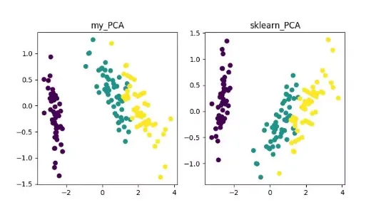
PCA Dimensionality Reduction Algorithm Demonstration
Of course, although this algorithm is classic and commonly used, its shortcomings are also very obvious. It can effectively eliminate linear correlations, but its performance deteriorates when faced with higher-order correlations; at the same time, the implementation of PCA assumes that the main features of the data are distributed in orthogonal directions, so PCA’s effectiveness will be greatly reduced for directions with large variances in non-orthogonal directions.
05 Other Dimensionality Reduction Algorithms and Code Locations
-
KPCA (Kernel PCA)
KPCA is a product of combining kernel techniques with PCA. Its main difference from PCA lies in the use of a kernel function when calculating the covariance matrix, which is the covariance matrix after mapping through the kernel function.
Introducing kernel functions can effectively solve the problem of nonlinear data mapping. KPCA can map nonlinear data to high-dimensional space and then use standard PCA to map it to another low-dimensional space.
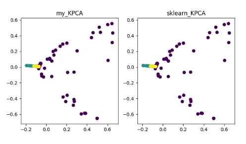
KPCA Dimensionality Reduction Algorithm Demonstration
For detailed content, please refer to “Python Machine Learning” on Feature Extraction—kPCA:
https://blog.csdn.net/weixin_40604987/article/details/79632888
Code location:
https://github.com/heucoder/dimensionality_reduction_alo_codes/blob/master/codes/PCA/KPCA.py
-
LDA (Linear Discriminant Analysis)
LDA is a technique that can be used for feature extraction, aiming to project in the direction that maximizes inter-class differences and minimizes intra-class differences, to effectively separate different classes of samples for tasks such as classification. LDA can improve computational efficiency in data analysis processes and reduce overfitting caused by the curse of dimensionality for models that have not been regularized.
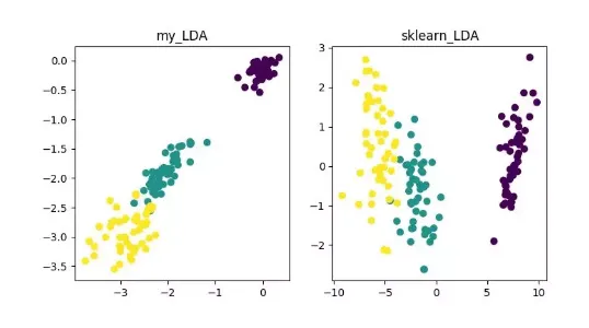
LDA Dimensionality Reduction Algorithm Demonstration
For detailed content, please refer to “Dimensionality Reduction—Linear Discriminant Analysis (LDA)”:
https://blog.csdn.net/ChenVast/article/details/79227945
Code location:
https://github.com/heucoder/dimensionality_reduction_alo_codes/tree/master/codes/LDA
-
MDS (Multidimensional Scaling)
MDS is a traditional dimensionality reduction method that represents the perceived preferences of research objects through intuitive spatial graphs. This method calculates the distance between any two sample points, ensuring that this relative distance is maintained after projecting into a low-dimensional space.
Since the MDS in sklearn uses an iterative optimization approach, both iterative and non-iterative implementations are provided below.
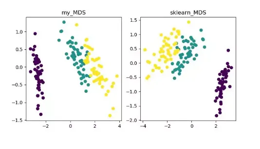
MDS Dimensionality Reduction Algorithm Demonstration
For detailed content, please refer to “MDS Algorithm”:
https://blog.csdn.net/zhangweiguo_717/article/details/69663452
Code location:
https://github.com/heucoder/dimensionality_reduction_alo_codes/tree/master/codes/MDS
-
ISOMAP
Isomap is an algorithm that can effectively address the shortcomings of the MDS algorithm on nonlinear structured datasets.
The MDS algorithm maintains the distance between samples after dimensionality reduction, while the Isomap algorithm introduces a neighborhood graph, connecting samples only with their neighboring samples, calculating the distances between nearest points, and then performing dimensionality reduction while preserving distances.
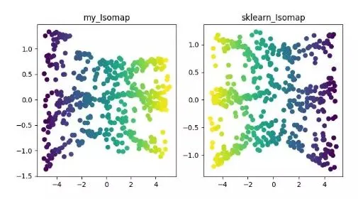
ISOMAP Dimensionality Reduction Algorithm Demonstration
For detailed content, please refer to “Isomap”:
https://blog.csdn.net/zhangweiguo_717/article/details/69802312
Code location:
https://github.com/heucoder/dimensionality_reduction_alo_codes/tree/master/codes/ISOMAP
-
LLE (Locally Linear Embedding)
LLE is a nonlinear dimensionality reduction algorithm. Its core idea is that each point can be approximately reconstructed by a linear combination of multiple neighboring points, and then project high-dimensional data into low-dimensional space while preserving the local linear reconstruction relationships between data points, i.e., having the same reconstruction coefficients. It performs significantly better than PCA when dealing with so-called manifold dimensionality reduction.
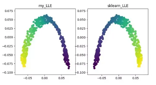
LLE Dimensionality Reduction Algorithm Demonstration
For detailed content, please refer to “LLE Principle and Derivation Process”:
https://blog.csdn.net/scott198510/article/details/76099630
Code location:
https://github.com/heucoder/dimensionality_reduction_alo_codes/tree/master/codes/LLE
-
t-SNE
t-SNE is also a nonlinear dimensionality reduction algorithm, very suitable for reducing high-dimensional data to 2D or 3D for visualization. It is an unsupervised machine learning algorithm that reconstructs the data trend in low dimensions (two or three) based on the original data trend.
The results below reference the source code and can also be implemented using TensorFlow (without manually updating parameters).
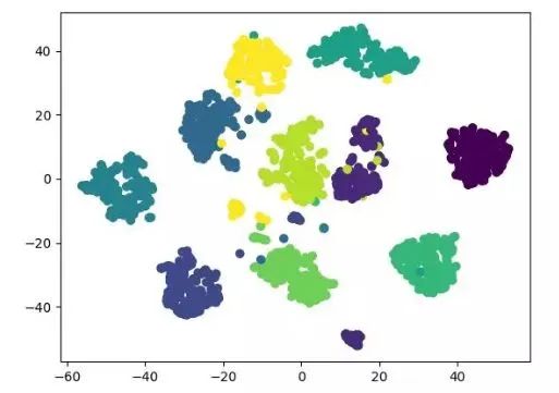
t-SNE Dimensionality Reduction Algorithm Demonstration
For detailed content, please refer to “Some Pits in Using t-SNE”:
http://bindog.github.io/blog/2018/07/31/t-sne-tips/
Code location:
https://github.com/heucoder/dimensionality_reduction_alo_codes/tree/master/codes/T-SNE
-
LE (Laplacian Eigenmaps)
LE is similar to the LLE algorithm and also constructs relationships between data from a local perspective. Its intuitive idea is that points that are related to each other (connected in the graph) should be as close as possible in the reduced dimensional space; in this way, a solution can be obtained that reflects the geometric structure of the manifold.
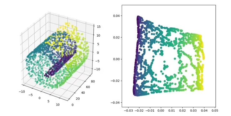
LE Dimensionality Reduction Algorithm Demonstration
For detailed content, please refer to “Laplacian Eigenmaps Dimensionality Reduction and Its Python Implementation”:
https://blog.csdn.net/HUSTLX/article/details/50850342
Code location:
https://github.com/heucoder/dimensionality_reduction_alo_codes/tree/master/codes/LE
-
LPP (Locality Preserving Projections)
LPP is a locality preserving projection algorithm. Its idea is similar to that of Laplacian Eigenmaps, where the core thought is to construct a projection mapping that best preserves the neighborhood structure information of a dataset, but unlike LE, LPP does not directly obtain projection results; it requires solving the projection matrix.
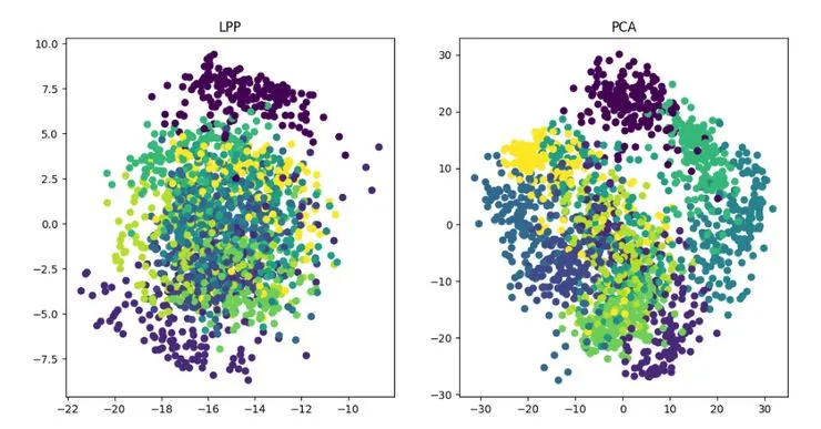
LPP Dimensionality Reduction Algorithm Demonstration
For details, please refer to “Detailed Explanation of Locality Preserving Projections (LPP)”:
https://blog.csdn.net/qq_39187538/article/details/90402961
Code location:
https://github.com/heucoder/dimensionality_reduction_alo_codes/tree/master/codes/LPP
* Author Information of the “dimensionality_reduction_alo_codes” Project
Heucoder, currently a master’s student in computer technology at Harbin Institute of Technology, is mainly active in the internet field, with the Zhihu nickname “Super Love Learning”. His GitHub homepage is: https://github.com/heucoder.
GitHub Project Address:
https://github.com/heucoder/dimensionality_reduction_alo_codes
This article is reprinted from: Meeting Robots.It is only used to convey and share more information and does not represent this platform’s endorsement of its views or responsibility for its authenticity. Copyright belongs to the original author. If there is any infringement, please contact us for deletion.
Editor /Fan Ruiqiang
Reviewed / Fan Ruiqiang
Rechecked / Fan Ruiqiang
Click below
Follow us