An interesting mathematical problem
The Fibonacci sequence originates from the famous “Rabbit Problem” proposed by the Italian mathematician Fibonacci in his book “Liber Abaci” published in 1202. This problem assumes: a pair of newborn rabbits can grow into adult rabbits after one month, and after another month, they can give birth to a pair of newborn rabbits, continuing to produce a pair of newborn rabbits every month thereafter. If no rabbits die within a year, how many pairs of rabbits can a pair of newborn rabbits reproduce in one year?
This seemingly simple breeding problem leads to an extremely interesting sequence: 1, 1, 2, 3, 5, 8, 13, 21, 34, 55, 89…
Sequence Rules and Characteristics
The rules of the Fibonacci sequence are very simple and elegant: The 1st and 2nd terms are both 1, and from the 3rd term onwards, each term is equal to the sum of the previous two terms.
Mathematically, this can be expressed as:
-
F(1) = 1
-
F(2) = 1
-
F(3) = F(1) + F(2)
-
F(n) = F(n-1) + F(n-2) (for n≥3)
Why does rabbit breeding follow such a rule? Each month, the number of rabbit pairs includes both adult and newborn rabbits. Every pair of rabbits (regardless of size) from the previous month becomes adult rabbits this month; at the same time, every pair of adult rabbits from the previous month gives birth to a pair of newborn rabbits this month.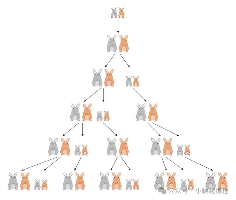
Real-World Case
The growth rate of the Fibonacci sequence is very fast, which has a painful lesson in history. In the early 20th century, British colonizers introduced European wild rabbits to Australia for hunting. Due to Australia’s warm climate, abundant grass, and lack of natural enemies, the rabbit population began to explode in a “Fibonacci sequence” manner, ultimately leading to a severe ecological disaster, forcing people to engage in a long “Rabbit War”.
In programming, we also need to be cautious of the rapid growth characteristics of the Fibonacci sequence. For example, the 46th term is 1,836,311,903, while the 47th term exceeds the range of a standard integer variable (over 2,147,483,647).
Algorithm Implementation: Iterative Solution
The solution to the Fibonacci sequence is a classic case for learning iterative algorithms. There are mainly two implementation methods:
1. Three-Variable Method
Using three variables f1, f2, and f3, we progress like a “worm crawling” through the sequence. The program first handles the special cases for n=1 and n=2, and the loop starts from i=3 until i=n, with each iteration calculating the new term f3 = f1 + f2; updating the values of f1 and f2 to prepare for the next iteration:
#include <iostream>using namespace std;int main() { // Input the number of Fibonacci sequence terms to calculate int n; cin >> n; // Handle special cases: the 1st and 2nd terms are both 1 if (n == 1 || n == 2) { cout << 1 << endl; return 0; // Directly return the result and end the program } // Initialize variables: // f1 represents F(n-2), initially the 1st term (1) // f2 represents F(n-1), initially the 2nd term (1) // f3 will store F(n), the current term to be calculated int f1 = 1, f2 = 1, f3; for (int i = 3; i <= n; i++) { // Start calculating from the 3rd term until the nth term f3 = f1 + f2; // Calculate the new term: F(n) = F(n-1) + F(n-2) // Update the values of the previous two terms for the next iteration: f1 = f2; // The original F(n-1) becomes the new F(n-2) f2 = f3; // The newly calculated F(n) becomes the new F(n-1) } cout << f3 << endl; // Output the nth Fibonacci number return 0; // Program ends normally}2. Two-Variable Method
#include<iostream>using namespace std;int main() { // Input the number of Fibonacci sequence terms to calculate int n; cin >> n; // Handle special cases: the 1st and 2nd terms of the Fibonacci sequence are both 1 if (n == 1 || n == 2) { cout << 1 << endl; return 0; } // Initialize variables: // f1 represents F(n-2), initially the value of the 1st term (1) // f2 represents F(n-1), initially the value of the 2nd term (1) // t is a temporary variable for swapping values int f1 = 1, f2 = 1, t; // Loop to calculate the Fibonacci numbers from the 3rd term to the nth term for (int i = 3; i <= n; i++) { // Save the current value of f2 into the temporary variable t, as f2 will be updated next t = f2; // Here f2 represents F(n-1), f1 represents F(n-2) f2 = f1 + f2; // Update f1 to the original value of f2 (saved in t) for the next iteration f1 = t; } // Output the nth Fibonacci number, after the loop ends, f2 stores the value of F(n) cout << f2 << endl; return 0;}Algorithm Comparison and Selection
|
Method |
Number of Variables |
Memory Usage |
Code Simplicity |
Applicable Scenarios |
|---|---|---|---|---|
|
Three-Variable Method |
3 |
Somewhat more |
Intuitive and easy to understand |
For beginners learning |
|
Two-Variable Method |
2 |
Less |
Concise and efficient |
Practical applications |
Batch Generation of the First 40 Fibonacci Terms
After mastering the basic iterative algorithm, let’s look at a more practical complete example—how to batch generate and beautifully display the first 40 terms of the Fibonacci sequence.
· Calculate the first 40 terms at once using an array to avoid repeated calculations;
· Use setw(12) to control output width, formatting five numbers per line for clear readability;
· Output the complete sequence at once for easy observation of the growth pattern of the Fibonacci sequence.
#include<bits/stdc++.h> // Include all standard library headersusing namespace std;int main() { int i; // Loop counter int f[50] = {0, 1, 1}; // Initialize Fibonacci array, first 3 terms known // Calculate Fibonacci sequence from the 3rd to the 40th term for (i = 3; i <= 40; i++) { f[i] = f[i-2] + f[i-1]; // Fibonacci sequence definition: F(n)=F(n-1)+F(n-2) } // Format output of the Fibonacci sequence for (i = 1; i <= 40; i++) { cout << setw(12) << f[i]; // Each number occupies 12 character widths if (i % 5 == 0) { // After outputting 5 numbers, move to the next line cout << endl; } } return 0; // Program ends normally}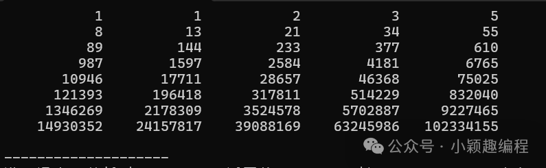
Conclusion
The Fibonacci sequence is not only an interesting mathematical problem but also a bridge connecting mathematics, nature, and computer science. From rabbit breeding to algorithm implementation, this simple yet elegant sequence continues to radiate its charm across multiple fields. By programming the Fibonacci sequence, we can not only gain a deep understanding of the essence of iterative algorithms but also appreciate the wonderful applications of mathematical rules in computer science.