💥💥💞💞Welcome to this blog❤️❤️💥💥
🏆Author’s Advantage: 🌞🌞🌞The blog content aims to be logically coherent and clear for the convenience of readers.
⛳️Motto: A journey of a hundred miles begins with a single step.
⛳️Gift to Readers
👨💻Conducting research involves a profound system of thought, requiring researchers to be logical and diligent, but effort alone is not enough; often leveraging resources is more important. Additionally, one must have innovative and inspiring ideas. When a philosophy teacher asks you what science is or what electricity is, do not find these questions amusing. Philosophy is the mother of science; it seeks to address ultimate questions and find those self-evident questions that only children would ask but you cannot answer. Readers are advised to browse in order to avoid suddenly falling into a dark maze without finding their way back. It may not reveal all the answers to your questions, but if it can evoke clouds of doubt in your mind, it may create a beautiful sunset of thoughts. If it brings you a storm in your spiritual world, then take the opportunity to brush off the dust that has settled on your ‘lying flat’ state.
Perhaps, after the rain, the sky will be clearer…….🔎🔎🔎
💥1 Overview
-
Core Principles and Structure of Filtering Methods
1.1 Federated Kalman Filtering (FKF)
Definition: FKF is a distributed filtering variant proposed by Carlson in 1998, employing a “divide-and-conquer” strategy.
Structure:
Composed of several sub-filters (local processors) and a main filter (global fusion center).
Sub-filters independently process local sensor data (e.g., radar, GNSS), while the main filter integrates the outputs of the sub-filters through information distribution principles.
Information Distribution Principle:
Dynamic information distribution: The information quantity of the state equation is represented by the inverse matrix of the process noise covariance Q-1, and the observation information quantity is represented by the inverse of the measurement noise covariance R-1.
Global fusion: The main filter weights the estimates of the sub-filters according to information weights (e.g., P-1) to generate the globally optimal trajectory.
Advantages: Strong fault tolerance (local failures do not affect the global system), distributed computational load.
1.2 Centralized Kalman Filtering (CKF)
Definition: A traditional single-center architecture where all sensor data (e.g., radar point clouds, GPS coordinates) is transmitted to a central processor for unified filtering.
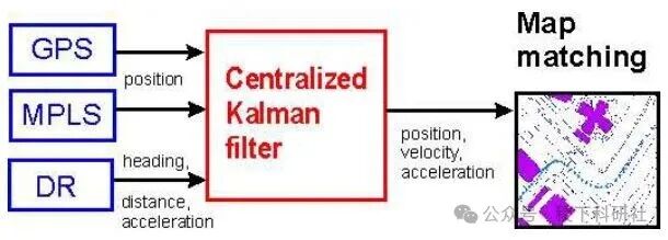

Principle:
Based on state-space models: The state equation describes the motion of the target (position, velocity), and the observation equation relates to sensor measurements.
Recursive prediction-update: The Kalman gain K balances the weights of the predicted values and the measured values to minimize the posterior error covariance.
Limitations:
High communication overhead (requires transmission of raw data), risk of single-point failure.
Computational complexity grows as O(n3) with the number of sensors, making it difficult to scale.
1.3 Decentralized Kalman Filtering (DKF)
Definition: No central node; sensors communicate with neighbors to collaboratively estimate the state.
Core Mechanism:
Prediction-correction two-step iteration:
Prediction: Each node predicts the current state based on the previous state and process noise.
Correction: Updates the state by exchanging information (e.g., local estimates, covariance) with neighbors.
Consensus optimization: Reformulates state estimation as a distributed optimization problem, using algorithms like ADMM to reduce communication costs.
Variants:
Olfati-Saber (2007) proposed three algorithms: DKF based on consensus filtering, continuous-time DKF, and iterative consensus DKF, supporting heterogeneous sensor networks.
-
Method Comparison: Performance and Applicable Scenarios
Dimension
Centralized (CKF)
Federated (FKF)
Distributed (DKF)
Structure: Star topology (single center) Tree topology (main-sub filter) Mesh topology (nodes interconnected equally)
Accuracy: Theoretically optimal (global information) Close to optimal (information weighted fusion) Dependent on communication topology
Robustness: Single-point failure leads to collapse Strong fault tolerance (local isolation) High fault tolerance (no central node)
Computational Load: Heavy burden on central node Parallel sub-filters, lightweight main filter Load balancing
Communication Overhead: High (transmission of raw data) Medium (transmission of local estimates) Low (neighbor exchange of summary information)
Applicable Scenarios: Small-scale fixed systems (e.g., laboratory benchmarks) Multi-source heterogeneous systems (e.g., INS/GPS integrated navigation) Large-scale dynamic networks (drone swarms, vehicle networks)
Key Differences:
CKF’s global optimality comes at a high resource cost;
FKF balances accuracy and complexity through hierarchical fusion;
DKF sacrifices communication efficiency for scalability, suitable for resource-constrained scenarios.
-
Practical Applications in Radar/Sensor Trajectory Estimation
3.1 FKF Application Cases
INS/GPS/TAN Integrated Navigation System:
Problem: The state vector dimensions of Inertial Navigation (INS), GPS, and Terrain-Aided Navigation (TAN) differ, making direct fusion difficult.
FKF Solution:
Sub-filters process INS, GPS, and TAN data separately, while the main filter fuses the outputs to generate a global trajectory.
Utilizes local state expansion/compression techniques to address dimensional differences, with intelligent filtering cycles adapting to dynamic environments.
Effect: Improved fault tolerance, adaptable to sudden trajectory changes (e.g., aircraft maneuvers).
Autonomous Driving Multi-Sensor Fusion:
Scenario: LiDAR, cameras, and GNSS for collaborative positioning.
FKF Improvement: Federated data-driven architecture (e.g., KalmanNet-RNN) estimates sensor uncertainty and shares local states through V2X communication.
Advantages: Avoids sharing raw data, protecting privacy while enhancing positioning accuracy.
3.2 CKF Application Cases
Shipboard Combat Command System:
Scenario: Aircraft carrier fuses data from multiple radars to track target trajectories.
CKF Solution: Central processor integrates radar point clouds, heading, and acceleration data to output high-precision trajectories.
Effect: Achieves optimal estimation when resources are sufficient, aiding critical military decisions.
Radar Target Tracking Simulation:
Verification: Simulates uniform and serpentine maneuvering target trajectories in MATLAB, using CKF as a benchmark to compare other methods.
Results: CKF maintains high accuracy under measurement noise standard deviations (distance 40m, azimuth 0.04rad).
3.3 DKF Application Cases
Drone Swarm Cooperative Detection:
Scenario: Multiple drones equipped with radars searching for moving targets.
DKF Solution:
Each drone performs local filtering and exchanges position covariance with neighbors via ADMM.
Consensus optimization achieves distributed trajectory prediction (e.g., target dive maneuvers).
Advantages: Reduces communication bandwidth requirements by 60%, adaptable to dynamic network topologies.
Intelligent Transportation Systems (ITS):
Scenario: Roadside radars monitoring vehicle trajectories.
DKF Implementation:
Nodes communicate only with adjacent intersection radars to collaboratively estimate regional traffic trajectories.
In the event of sudden obstacles (e.g., pedestrians crossing), trajectory corrections are completed within 200ms.
-
Frontier Trends and Challenges
4.1 Fusion Learning and Optimization
Federated Learning + FKF:
Jointly training local Kalman gain models in vehicular networks to improve noise estimation accuracy.
DKF Communication Optimization:
ADMM framework compresses the amount of exchanged information, addressing communication bottlenecks in large-scale networks.
4.2 Nonlinear Extensions
EKF/FKF Hybrid:
In intelligent reflective surface communication perception systems, EKF locally linearizes the target motion model, while FKF fuses data from multiple base stations.
Particle Filtering Assistance:
For complex maneuvering targets (e.g., aerial flips), particle filtering generates local trajectories, while DKF achieves multi-sensor consensus.
4.3 Challenges
FKF: The design of information distribution factors relies on experience, requiring adaptive weight algorithms.
DKF: Stability under non-Gaussian noise is insufficient, necessitating robust optimization.
Real-time Requirements: Radar trajectory estimation requires millisecond-level responses, making hardware acceleration (e.g., FPGA) crucial.
Conclusion
In the field of radar/sensor trajectory estimation:
CKF is suitable for resource-rich, precision-prioritized fixed scenarios (e.g., shipboard systems);
FKF balances performance and fault tolerance in multi-source heterogeneous systems (e.g., integrated navigation);
DKF provides scalable solutions for dynamic networks (drone swarms, vehicular networks).
Future research will focus on adaptive information distribution, communication-computation collaborative optimization, and enhancing nonlinear scenarios to meet the demands of high-maneuverability target tracking.
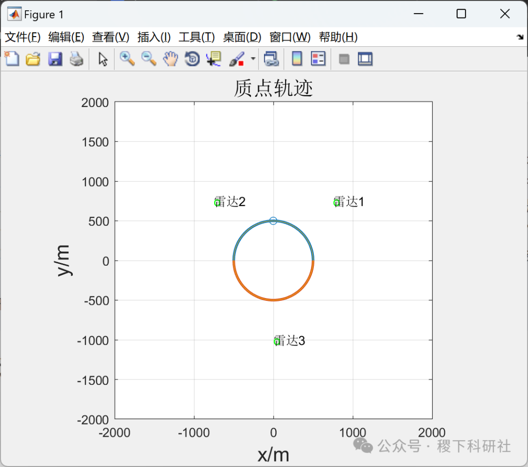
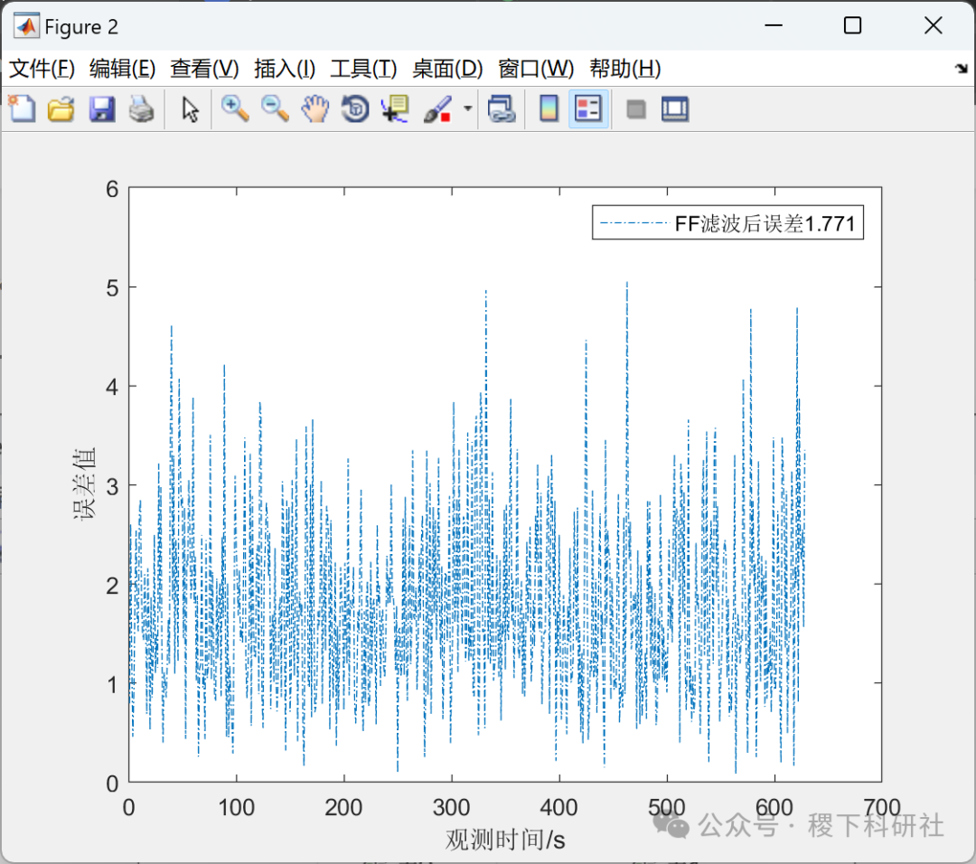
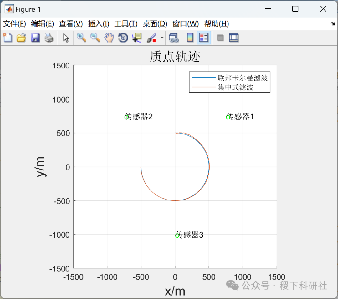
📚2 Operational Results
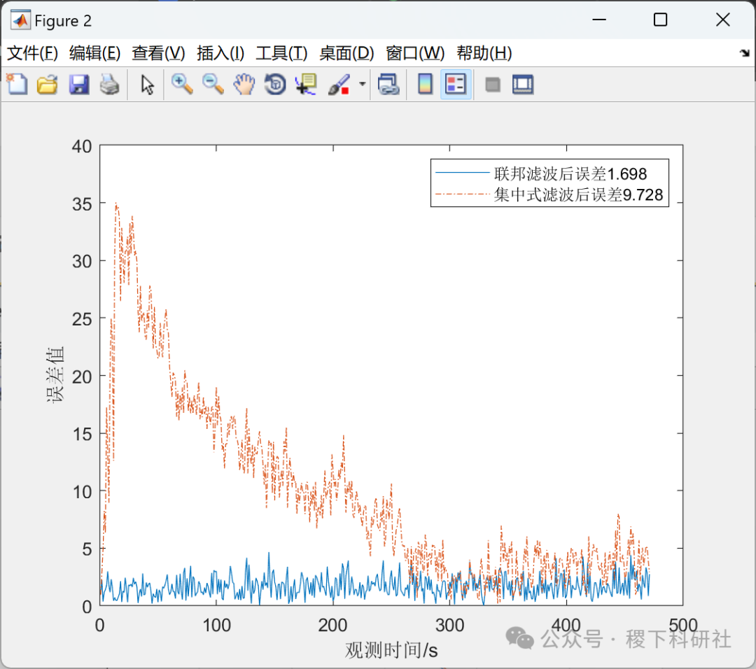
2.1 Federated Kalman Filter


2.2 Decentralized Kalman Filter


Some Code:
% Radar positions
radar_1 = [750 750];
radar_2 = [-750 750];
radar_3 = [0 -1000];
radar1_noise = 3;
radar2_noise = 1;
radar3_noise = 4;
% True measurement signals
radar1_ture_measuremnet = sqrt((radar_1(1)-x_ture_traj).^2 + (radar_1(2)-y_ture_traj).^2 );
radar2_ture_measuremnet = sqrt((radar_2(1)-x_ture_traj).^2 + (radar_2(2)-y_ture_traj).^2 );
radar3_ture_measuremnet = sqrt((radar_3(1)-x_ture_traj).^2 + (radar_3(2)-y_ture_traj).^2 );
% Noisy measurements
radar1_noise_measuremnet = radar1_ture_measuremnet + radar1_noise * randn(1,size(radar1_ture_measuremnet,2));
radar2_noise_measuremnet = radar2_ture_measuremnet + radar2_noise * randn(1,size(radar2_ture_measuremnet,2));
radar3_noise_measuremnet = radar3_ture_measuremnet + radar3_noise * randn(1,size(radar3_ture_measuremnet,2));
%%
% Federated filter structure with FR (fusion reset structure)
% Federated filter with three sub-filters and one main filter
beta_M = 0;
N = 3;
beta_i = 1/N;% Each sensor is assigned the same weight
Q_process_noise_system = diag([2 2]);% System process noise, as required by the problem
P_cov_system = diag([1000 1000 ]);% Initial system covariance, arbitrarily given
X_init_state = [0;500];% Initial target position
%%%%%%%%%%%%%%%%%%%%%%%%%%%%1. Information distribution and reset%%%%%%%%%%%%%%%%%%%%%%%%%%%%%%%%%%%%%
🎉3 References
Some content in this article is sourced from the internet, and references will be noted. If there are any inaccuracies, please feel free to contact for removal.
[1] Tang Juan. Research on Key Technologies of Integrated Navigation Based on Federated Strong Tracking Kalman Filtering [D]. Shandong University, 2019.
[2] Tang Juan. Research on Key Technologies of Integrated Navigation Based on Federated Strong Tracking Kalman Filtering [D]. Shandong University, 2018. DOI: CNKI:CDMD:2.1018.110701.
[3] Zhao Hangzhou. Research on Fault Diagnosis of Multi-Sensor Integrated Navigation Based on Federated Kalman Filtering [D]. Beijing Institute of Technology, 2017.
[4] Deng Hubin, Zhang Lei, Wu Ying, et al. Research on Trajectory Estimation Based on Kalman Filtering Algorithm [J]. Sensors and Microsystems, 2012, 31(5):4. DOI: 10.3969/j.issn.1000-9787.2012.05.002.
🌈4 MATLAB Code Implementation
Reply in the public account background: Program download