In the development of ECU application software models, the first-order low-pass filter is one of the most commonly used filtering methods, because it can:

• Eliminate “unreliable high-frequency components” from sensor or bus signals

Raw values such as wheel speed, accelerator pedal position, and battery voltage are superimposed with PWM switching noise, ADC quantization noise, or electromagnetic coupling spikes. The first-order low-pass filter attenuates these high-frequency energies by more than 20 dB with a configurable cutoff frequency (typically 1–20 Hz), allowing the subsequent control laws to see signals that are “physically real” rather than “sampling noise.”

• Prevent the controller from “overreacting”

For engine torque control, cruise PID, EPS current loop, etc., if unfiltered signals are used directly, the differential and proportional terms will produce large output jumps for each spike, causing actuator jitter, audible noise from the motor, and even torque oscillation. Low-pass filtering smooths out changes outside the “allowed bandwidth,” allowing the controller to only track the real trend, enabling higher system gain without oscillation.

This article focuses not on the theoretical research of first-order low-pass filtering, but on the application process of ECU application layer software model development, thus focusing on: how to set the filtering coefficient? How to analyze the filtering delay time?

1 First-Order Low-Pass Filter Model

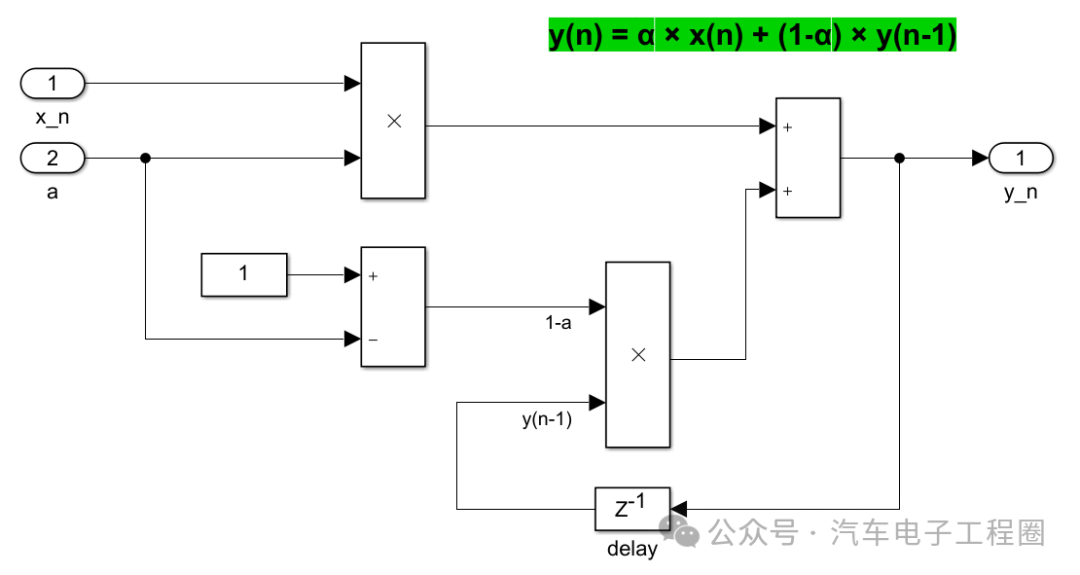
The discrete equation of the first-order low-pass filter is:

y(n) = α × x(n) + (1-α) × y(n-1)

Where:

• x(n): The raw signal value of the current sampling period.

• y(n): The filtered signal value of the current period.

• y(n-1): The filtered result of the previous period (historical value that needs to be saved).

• α: The filtering coefficient (0 < α < 1), where a larger α results in weaker filtering effect and faster response.

The Simulink model built is shown below:

Here we provide a signal input and a strong filtering coefficient to observe the effect, as shown in the figure below:

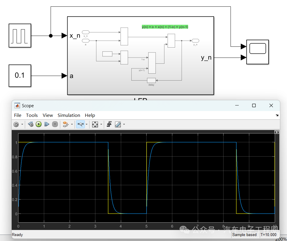
In the above figure, the yellow line represents the raw signal, and the blue line represents the filtered signal. There are two questions: Does the filtering effect meet expectations? Does the filtering delay meet expectations?

2 How to Set the Filtering Coefficient α

For the first question, it concerns the setting of the filtering coefficient α, how to set it?

The value of α directly determines the filtering effect (smoothness) and response speed (delay), and should be designed based on the signal bandwidth and noise frequency:

Step 1: Determine the cutoff frequency fc. The cutoff frequency fc is a core indicator of the filtering system and must satisfy:

• It should be below the effective bandwidth of the signal (to retain the main changing components of the signal).

• It should be above the main frequency of the noise (to filter out high-frequency noise).

If the signal is a slowly changing water temperature (effective bandwidth <1Hz), and the noise is mainly above 10Hz, fc=2Hz can be selected; if the signal is a dynamically changing air pressure (effective bandwidth <10Hz), and the noise is mainly above 50Hz, fc=10Hz can be selected.

Step 2: Calculate the filtering coefficient α based on the cutoff frequency fc. Assuming a system sampling period (10ms) and a desired cutoff frequency fc=10Hz, then according to α=1-exp(-T/τ)≈T/(T+τ) (when T<<τ, it is approximate), where:

• T: Sampling period (10ms = 0.01s).

• τ: Time constant (τ=1/(2πfc)).

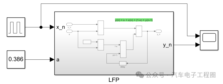
Since the cutoff frequency fc=10Hz, τ≈0.0159s, thus α≈0.01/(0.01+0.0159)≈0.386.

3 How to Analyze Filtering Delay

The delay introduced by the first-order low-pass filter mainly depends on the filtering coefficient α and the operating period Ts. The delay is usually represented by the time constant τ, which is defined as the time for the output to reach 63% of the step response.

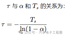
This relationship is very important as it establishes a bridge between the ECU’s operating period Ts, filtering coefficient α, and time constant τ. Regarding the measurement of delay, in engineering, we usually care about two points:

• The time to reach 63.2%: This is the time constant <span><span>τ</span></span> itself.

• The time to reach 50% (step response delay): This time<span><span>t{50}</span></span> better represents the delay of the signal “center.” Its relationship with the time constant is: t{50} = ln(2) * τ ≈ 0.693 * τ.

When the filtering coefficient<span><span>α</span></span> is very small (for example, <span><span>α<0.3</span></span>), <span><span>ln(1-α)≈-α</span></span>, thus the formula can be simplified to: τ≈Ts/α. This approximation is very accurate and intuitive when <span><span>α</span></span> is very small. It implies:

• When the operating period<span><span>Ts</span></span> is fixed, <span><span>α</span></span> smaller results in a larger time constant<span><span>τ</span></span> and greater delay.

• When the filtering coefficient<span><span>α</span></span> is fixed, the longer the operating period<span><span>Ts</span></span>, the greater the delay.

Based on this, we will calculate the delays caused by different filtering coefficients α when the operating period Ts=10ms, as shown in the table below:

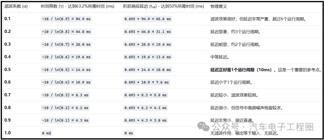
From this, we can see that the essence of choosing α is to make a trade-off between filtering effect (anti-noise capability) and response speed (delay magnitude). A filtering effect with α=0.1 is smooth but has a delay of up to 65.8ms, while α=0.8 has a delay of only 4.3ms but a minimal filtering effect. Engineers must carefully choose parameters based on specific applications (such as engine control, body stability systems, battery management) according to the requirements for real-time performance and stability.

Creating is not easy, please like, save, and follow! (Qian Yixing Renamed Automotive Electronics Engineering Circle) Automotive R&D group chat, interested friends please add the group owner: prOmiseyes, note: company + position to join the group. Limited to automotive practitioners.

Articles in the ECU application layer software model series are continuously updated, teaching you application layer development from scratch:

• An example of building an ECU application layer software model 1 (qq.com)
• How to automatically generate code for ECU application layer software model 2 (qq.com)
• How to run ECU application layer software periodically 3 (qq.com)
• Code generation configuration related to ECU application layer software model and hardware 4 (qq.com)
• Data dictionary DD of ECU application layer software model 5 (qq.com)
• Data dictionary storage class of ECU application layer software model 6 (qq.com)
• Fixed-point implementation of ECU application layer software model 7 (qq.com)
• Five fixed-point implementation methods of ECU application software model 8 (qq.com)
• Custom storage class of ECU application layer software model 9 (qq.com)
• Summary of model generation code of ECU application layer software model 10 (qq.com)
• CAN reception of ECU application layer software model 11 (qq.com)

• Data stream of CAN message reception in ECU application layer model 12
• How to leverage AI in ECU software development? Application of Kimi in MBD development environment 13

• Unit test coverage CC, DC, and MCDC detailed explanation of ECU application layer software model 14

• Application and principles of calibration quantity and observed quantity in ECU application layer model development 15

• Usage of for loop in ECU application layer model development 16

• Usage of if-else in ECU application layer model development 17
• Initialization function in ECU application layer model development 18

• Counter in ECU application layer model development 19

• Basics of Assignment module in ECU application layer model development 20

• Application of Delay module in ECU application layer model development 21

• ECU application layer model development: If-else VS switch-case 22

• Simulink.Signal in ECU application layer model development 23

• Data overflow handling in ECU application layer model development 24

• Disasters caused by Delay in ECU application layer model development 25

• Usage of Tapped Delay in ECU application layer model development 26