Robotic servo joints, as the core execution components of robots, require a design process that considers multiple dimensions such as mechanical structure, electrical control, sensor fusion, and dynamic optimization. The following systematically elaborates on the design process of robotic servo joints through six stages: requirement analysis, system design, hardware selection, software development, simulation verification, and testing optimization.
1. Requirement Analysis and Function Definition
1.1 Clarification of Application Scenarios
At the initial design stage, it is essential to clarify the application scenarios of the servo joints, such as industrial handling, medical rehabilitation, humanoid robots, or quadruped bionic robots. Different scenarios have significantly different requirements for joint load capacity, motion range, response speed, and precision:
• Industrial Handling: Requires high load (e.g., over 50kg), low-speed stability (0.1-1m/s), and repeat positioning accuracy of ±0.1mm.
• Humanoid Robots: Requires lightweight (joint mass < 1kg), high dynamic response (acceleration > 5m/s²), and multi-degree-of-freedom coordination.
• Quadruped Bionics: Requires impact-resistant design, low power consumption (endurance > 2 hours), and terrain adaptability.
1.2 Quantification of Performance Indicators
Based on scenario requirements, key performance indicators are quantified:
• Motion Parameters: Maximum speed (e.g., 300rpm), joint travel (e.g., ±90°), acceleration (e.g., 10rad/s²).
• Force/Torque Parameters: Continuous output torque (e.g., 5Nm), peak torque (e.g., 15Nm), backlash (< 0.1°).
• Environmental Adaptability: Operating temperature (-20℃~60℃), protection level (IP65 or above), electromagnetic compatibility (EMC).
1.3 Identification of Constraints
Identify design constraints, including cost budget (e.g., single joint cost < $500), size limitations (e.g., diameter < 100mm), interface standards (e.g., EtherCAT bus), and certification requirements (e.g., CE, UL).
2. System Architecture Design
2.1 Mechanical Structure Design
2.1.1 Drive Scheme Selection
• Direct Drive Scheme: Suitable for high dynamic, low load scenarios (e.g., quadruped robots), directly driven by frameless torque motors, eliminating reducer backlash, but requires high power density motors (e.g., peak power > 500W).
• Reducer Scheme: Uses harmonic reducers (e.g., HD series) or planetary reducers to enhance output torque (e.g., torque amplified 100 times at a reduction ratio of 100:1), but requires balancing inertia matching (reducer inertia < 5 times motor inertia).
2.1.2 Structural Optimization
• Lightweight Design: Uses 7075 aluminum alloy or carbon fiber composite materials, reducing joint mass by over 30%.
• Thermal Management: Integrates liquid cooling channels or phase change materials (PCM), controlling motor temperature rise < 80℃.
• Sealing Design: Uses double-lip seals or magnetic fluid seals, achieving a protection level of IP67.
2.2 Electrical System Design
2.2.1 Driver Selection
• Power Density: Select drivers with peak current > 20A and switching frequency > 20kHz (e.g., Elmo Gold Twitter series).
• Control Mode: Supports three-loop control of current loop (20kHz), speed loop (5kHz), and position loop (1kHz), with feedforward compensation in the position loop (e.g., acceleration feedforward coefficient 0.2).
2.2.2 Sensor Configuration
• Position Sensor: Uses a 23-bit absolute encoder (e.g., Renishaw ATOM series) with a resolution of 0.0007°.
• Force/Torque Sensor: Integrates strain gauge torque sensors (range ±20Nm, accuracy ±0.1%FS).
• Temperature Sensor: PT100 thermistor to monitor motor winding temperature.
2.3 Control Algorithm Design
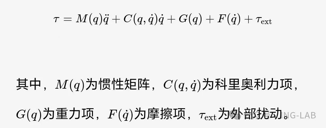
2.3.1 Dynamic Model
Establish the joint dynamic equations:
2.3.2 Control Strategy
• PID Control: The position loop uses proportional-derivative (PD) control, the speed loop uses proportional-integral (PI) control, and the current loop uses proportional (P) control.
• Adaptive Control: Introduces friction compensation (e.g., Stribeck model) and inertia identification (e.g., recursive least squares method).
• Robust Control: Uses H∞ control or sliding mode control to suppress model uncertainties (e.g., load sudden changes).
3. Hardware Selection and Integration
3.1 Motor Selection
• Type Selection: Choose between brushless DC motors (BLDC) or permanent magnet synchronous motors (PMSM) based on speed requirements. For high-speed scenarios (e.g., >1000rpm), use PMSM; for low-speed high-torque scenarios, use BLDC.
• Parameter Matching: The motor rated torque must be greater than 1.5 times the maximum required torque of the joint, and the peak torque must exceed 3 times.
3.2 Reducer Selection
• Type Comparison: Harmonic reducers (backlash < 0.1°) are suitable for high-precision scenarios, while planetary reducers (30% lower cost) are suitable for general scenarios.
• Lifetime Verification: Ensure the reducer’s lifetime > 5 years through L10 lifetime calculations (e.g., 10^7 cycles).
3.3 Driver Integration
• Interface Matching: The driver must support CAN, EtherCAT, or RS485 buses, with communication cycles < 1ms with the main controller.
• Safety Features: Integrate overcurrent protection (e.g., 15A overcurrent threshold), overvoltage protection (e.g., 60V overvoltage threshold), and emergency stop (E-Stop) functions.
4. Software Development and Debugging
4.1 Embedded Software Architecture
• Layered Design: Divided into hardware abstraction layer (HAL), driver layer, control algorithm layer, and application layer.
• Real-time Assurance: Use RTOS (e.g., VxWorks or FreeRTOS) with task scheduling cycles < 1ms.
4.2 Debugging Toolchain
• Data Acquisition: Connect a logic analyzer (e.g., Saleae Logic) via JTAG or SWD interfaces to collect current and position signals.
• Parameter Tuning: Use the Ziegler-Nichols method to tune PID parameters, with overshoot < 5% and adjustment time < 100ms.
5. Simulation and Verification
5.1 Dynamic Simulation
• Model Building: Establish the joint dynamic model in MATLAB/Simulink to verify the effect of friction compensation (e.g., friction reduced by 40%).
• Coupling Analysis: Analyze the impact of inter-joint coupling inertia on system stability through multibody dynamics simulation (e.g., ADAMS), with coupling stiffness > 1000N/m.
5.2 Hardware-in-the-Loop (HIL) Testing
• Testing Platform: Build a dSPACE real-time simulation system to simulate load sudden changes (e.g., step from 0 to 10Nm) and external disturbances (e.g., 0.1g vibration).
• Performance Indicators: Verify position tracking error < 0.1° and torque control accuracy < ±0.5%FS.
6. Testing and Optimization
6.1 Performance Testing
• Test Bench Testing: Continuously run 10^6 cycles on a fatigue testing machine to verify joint lifespan (e.g., backlash change < 0.05°).
• Environmental Testing: Test startup time (e.g., < 2s) and power loss (e.g., < 5W) in a temperature chamber at -20℃~60℃.
6.2 Optimization Iteration
• Lightweight Optimization: Reduce material usage by 15% through topology optimization (e.g., Altair OptiStruct).
• Control Parameter Optimization: Use genetic algorithms to optimize PID parameters, shortening adjustment time by 30%.
7. Case Studies
7.1 Industrial Handling Robot Joint
• Design Features: Uses harmonic reducer (reduction ratio 80:1) + PMSM motor, peak torque 12Nm, repeat positioning accuracy ±0.05mm.
• Application Effect: In automotive welding production lines, single joint failure rate < 0.1%, maintenance cycle extended to 5000 hours.
7.2 Humanoid Robot Knee Joint
• Design Features: Direct drive frameless motor (peak power 300W) + elastic actuator, natural frequency 5Hz, energy efficiency improved by 20%.
• Application Effect: In gait planning, joint torque fluctuation < 1Nm, walking stability improved by 40%.
8. Future Trends
8.1 Material Innovation
• Carbon Fiber Composites: Joint mass reduced by 50%, stiffness increased by 3 times.
• Shape Memory Alloys: Achieve adaptive stiffness adjustment (e.g., stiffness variation range 100:1).
8.2 Control Technology Upgrades
AI-driven control: Achieve parameter self-tuning through deep reinforcement learning (e.g., PPO algorithm), with response speed improved by 50%.
• Digital Twin: Build a digital model of the joint for predictive maintenance (e.g., fault warning 72 hours in advance).
8.3 Standardization and Modularity
• Interface Standardization: Promote ROS 2.0 middleware for plug-and-play joints.
• Design Reuse: Establish a joint parameter library (e.g., torque-speed-inertia database), improving design efficiency by 60%.
The design of robotic servo joints requires interdisciplinary collaboration, forming a closed loop from requirement analysis to testing optimization. In the future, with the development of materials science, artificial intelligence, and the industrial internet, servo joints will evolve towards higher precision, lighter weight, and greater intelligence, providing core support for the robotics industry.