Previous article review:
【Industrial Robots | Key Points (I)】 Introduction & Mechatronic Structure
Chapter 3 Control Systems and Motion Control
Industrial Robot Controller
Classification: Based on openness, architecture classification
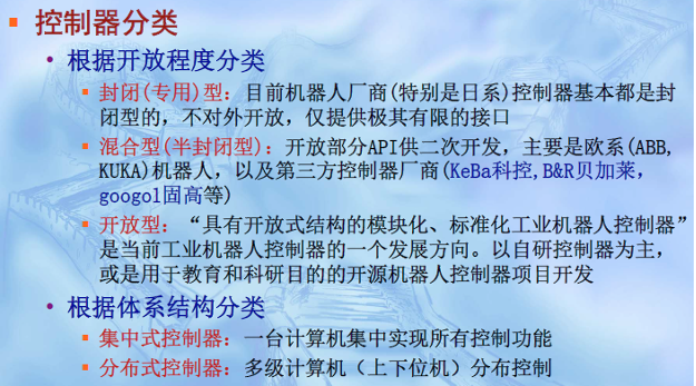
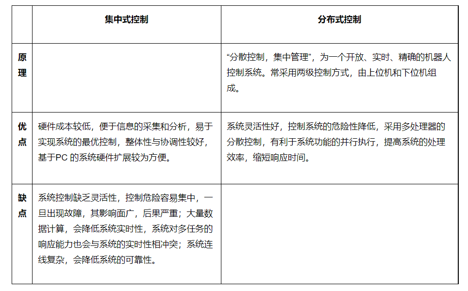
Centralized controller vs Distributed controller, principles, comparison
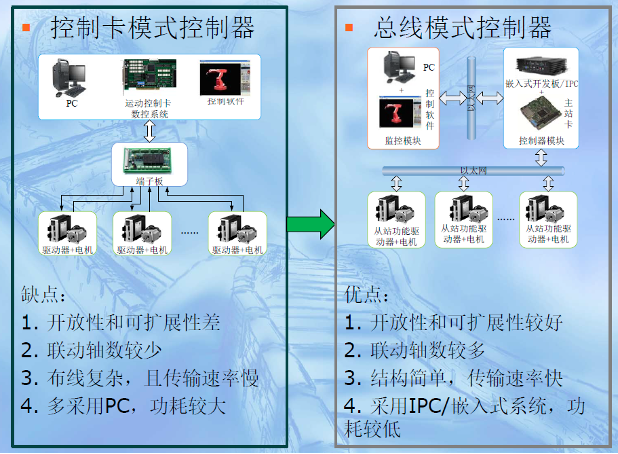
Interface forms of servo control: Pulse vs Bus, advantages and disadvantages comparison.
Interface forms of servo control:
-
Analog: Mostly required for high-speed and high-precision, accurate trajectory tracking scenarios.
-
Pulse/Direction: Low cost. The downside is step loss, poor anti-interference, and synchronization is a matter of luck.
-
Bus: EtherCAT, SERCOS, ProfiBus, ModBus, etc. Advantages include simple wiring, the more axes the easier the bus control; high real-time reliability, good system redundancy. Disadvantages include system complexity, high costs.
Motion Control of Industrial Robots
Forward Kinematics vs Inverse Kinematics; PTP vs CP; Concept of interpolation.
Forward Kinematics Problem: Given the joint angle vector, calculate the pose of the end effector relative to the reference coordinate system, known as forward kinematics (kinematic forward solution or Where problem). When teaching the robot, the robot controller performs forward kinematic calculations point by point.
Inverse Kinematics Problem: Given the initial and target (desired) poses of the end effector in the reference coordinate system, calculate the joint angle vector, known as inverse kinematics (kinematic inverse solution or How problem). During reproduction, the robot controller performs inverse kinematic calculations point by point and decomposes the vector to each joint of the manipulator.
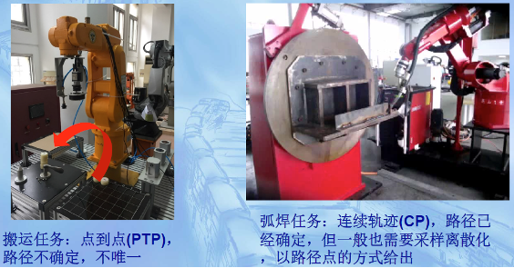
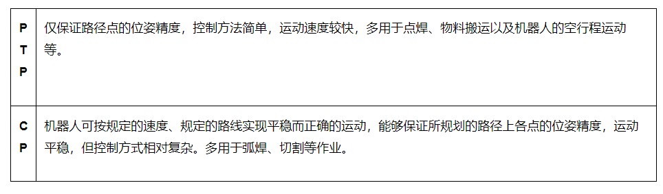
Point-to-Point Motion (PTP): PTP motion only cares about the start and target poses of the robot’s end effector, regardless of the trajectory between these two points.
Continuous Path Motion (CP): CP motion not only cares about the accuracy with which the robot’s end effector reaches the target point but must ensure that the robot can repeat the motion along the desired trajectory within a certain accuracy range.
Relationship: The realization of CP motion is based on PTP motion, achieved by using linear or circular trajectory interpolation calculations that meet accuracy requirements between adjacent points to achieve continuity of the trajectory.
Concept of Interpolation: When the robot reproduces, the main controller (host computer) retrieves each teaching point’s spatial pose coordinate values from memory point by point. By performing linear or circular interpolation calculations, it generates the corresponding path planning, and then converts the pose coordinate values of each interpolation point into joint angle values through inverse kinematic calculations, distributing them to each joint or joint controller (lower computer).
The classic three-loop control structure of robots, feedforward control
Control Forms of Industrial Robots (With or Without Feedback):
-
Open-loop Control: The robot model is incomplete, with problems such as noise and interference, leading to low control accuracy.
-
Closed-loop Control: Requires joint sensors to provide feedback signals for displacement, speed, and even acceleration.
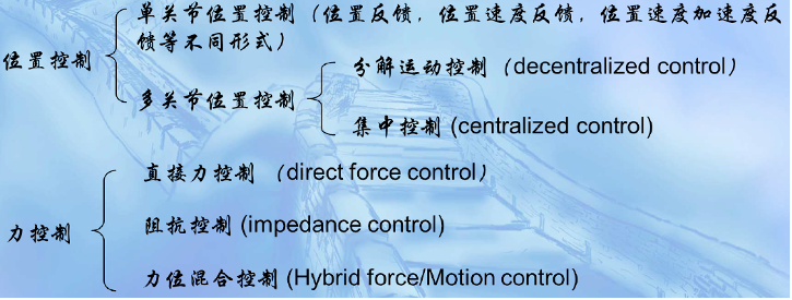
Control Methods of Industrial Robots
-
Position Control
-
Speed Control
-
Current Control, Force/Torque Control
-
Force/Position Hybrid Control
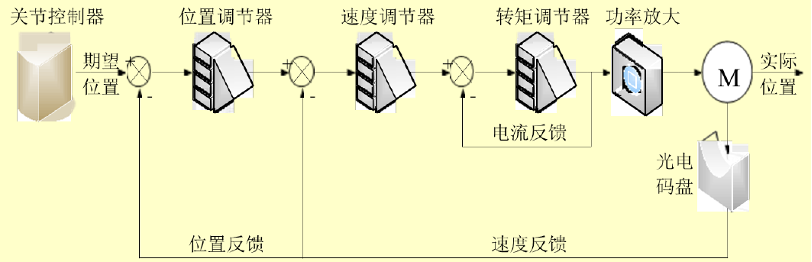
Classic Industrial Robot Control Loop Composition:
The three-loop (position, speed, current) structure of a single-axis robot arm, with each loop’s control law completed using PID control, and parameters already tuned. Generally, the current loop is not open to external access, and operators usually control the position loop through a teaching box or design corresponding control laws by combining position and speed loops.
Position control is the basic control task of industrial robots. The joint controller (lower computer) is the execution computer, responsible for closed-loop control of the servo motor and coordinating all joint movements.
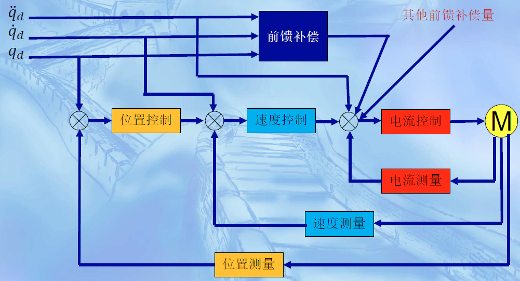
Feedforward Control: When the robot is in high-speed motion, the accuracy of position and speed feedback decreases significantly. At this time, feedforward compensation is used to improve tracking accuracy. Other nonlinear items (such as gravity, friction) can also be compensated in a similar manner.
Classification of Control Tasks of Industrial Robots (Based on Desired Control Quantity)
-
Position Control: High rigidity, or non-contact constraints, such as CP control (arc welding, spraying, etc.) and PTP control (spot welding, handling, palletizing, etc.)
-
Force (or Force-Position Hybrid) Control: Flexible control, with contact constraints, such as deburring, cutting, shaft-hole assembly, glass cleaning tasks
Chapter 4 Manual Operation and Teaching Reproduction
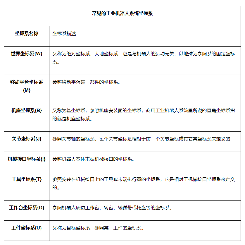
Motion Axes and Coordinate Systems
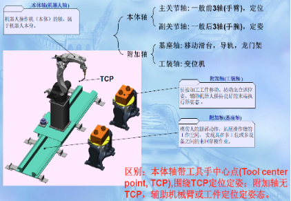
Definition and classification of motion axes
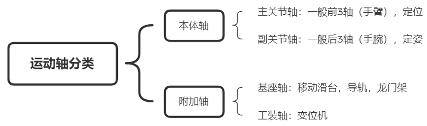
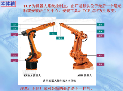
Body Axis: The axis of the robot manipulator (body), belonging to the robot itself.
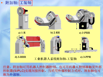
Additional Axis (Tool Axis): Moves and rotates the workpiece to the appropriate pose, assisting the robot in maintaining a good end effector posture.
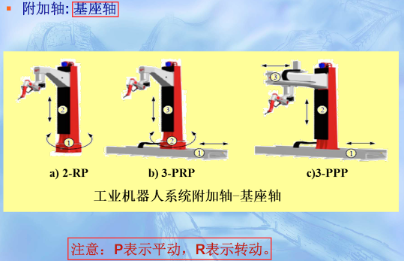
Additional Axis (Base Axis): Mimics human leg movements, expands the workspace of the manipulator, enabling it to shuttle between multiple workstations or devices.
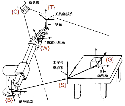
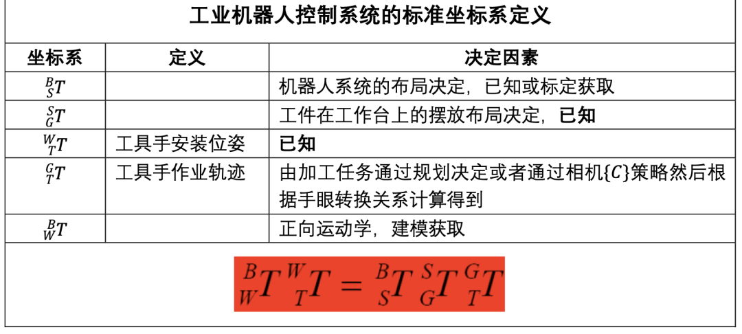
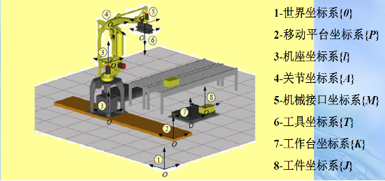
Definition of application system coordinate systems, motion chains, task processes
Manual Operation
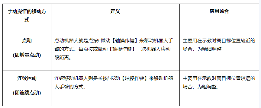
Movement methods: Jogging vs Continuous motion, application scenarios for both
Setting of TCP, six-point calibration steps

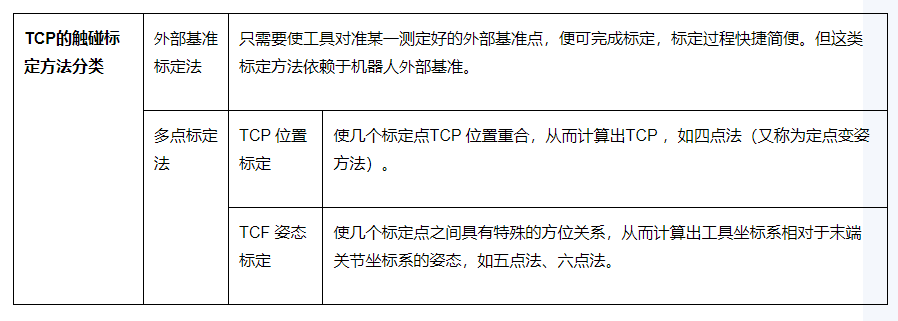
Six-point TCP Calibration Steps:
1) Find an accurate fixed point within the robot’s range of motion as a reference point.
2) Determine a reference point on the tool (preferably the tool center point TCP).
3) Move the tool reference point to touch the fixed point as closely as possible in four different tool postures. Note that the 4th point needs to be perpendicular to the fixed point.
4) The robot control cabinet can calculate the TCP position from the position data of the first four points and determine the TCP posture from the last two points.
5) Set the tool’s mass and center of gravity data according to the actual situation.
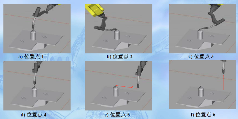
Figure 1 Six-point TCP Calibration Process
Note:
1) TCP calibration operations should focus on the secondary axis (wrist axis);
2) Reduce speed near the reference point to avoid collisions;
3) After TCP calibration, control point invariant motion tests can be conducted in a coordinate system outside the joint coordinate system to verify the calibration effect.
Basics of Teaching Operations
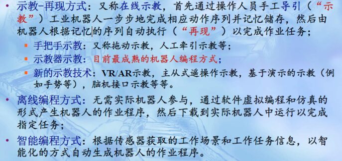
Programming methods: Teaching, offline programming, intelligent programming. Concepts
The three programming methods correspond to three generations of industrial robot technology!
Programming languages: Action level, Object level, Task level. Concepts. Differences
1) Action Level: Describes various operations centered on the robot’s end effector’s actions, requiring each action to be specified in the program. This is the most basic description method;
2) Object Level: Allows for a rough description of the actions of the operating objects, relationships between operating objects, etc. When using this language, it is essential to clearly describe the relationships between operating objects and the relationships between the robot and the operating objects. It is particularly suitable for assembly tasks;
3) Task Level: Directly specifies the operation content, requiring the robot to think while working. This is a high-level robot programming language.
Currently, most commercial robot programming languages are action-level, and each robot language is not standardized (but generally similar), while object-level and task-level are still in the experimental research stage or only targeted at specific applications.
Concept of teaching and reproduction, three elements of teaching
“Teaching”: Also known as guiding, it involves the operator directly or indirectly guiding the robot, step by step informing the robot of the actions and specific content it should complete according to actual work requirements. The robot memorizes this during the guiding process in the form of a program and stores it in the robot control device;
“Reproduction”: By replaying stored content, the robot can demonstrate the taught actions and assigned work content within a certain accuracy range. The program describes the robot’s work content in robot language, used to save teaching data and robot instructions generated during teaching operations.
Three elements of teaching:
-
Motion trajectory:
-
Point-to-Point (PTP) motion
-
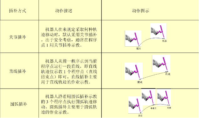
Continuous Path (CP) motion: Two types of paths, straight and circular, any complex path can be formed by combinations of straight lines and arcs
-
Classified by motion methods:
-
Working conditions (process conditions)
-
Work sequence (action sequence)
Three interpolation methods, differences
Five attributes of teaching points, specific definitions
Attributes of Teaching Points (or Program Points):
-
Position coordinates: Describes the 6 degrees of freedom (3 translational and 3 rotational) of the robot’s TCP
-
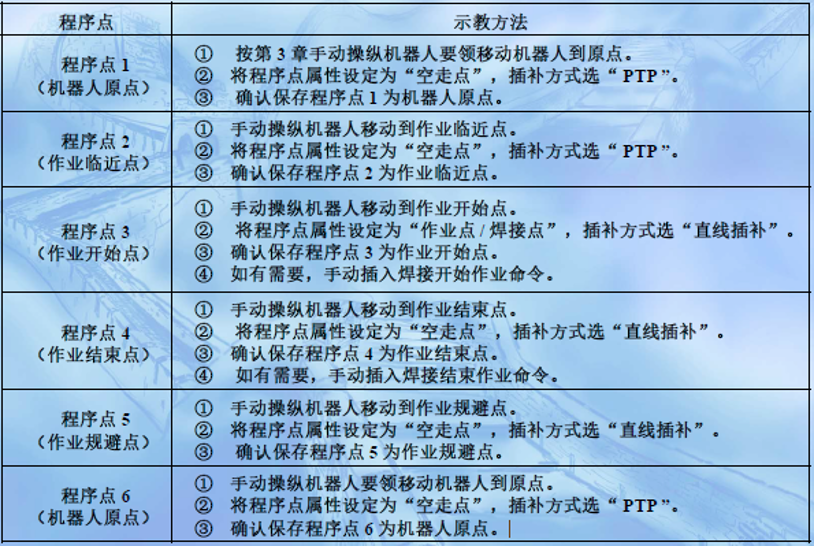
Interpolation method: The type of motion from the previous program point to the current program point during robot reproduction
-
Reproduction speed: The speed at which the robot moves from the previous program point to the current program point during reproduction
-
Empty motion point: The entire process of moving from the current program point to the next program point does not require implementation of work, used for teaching program points other than the work start point and intermediate points.
-
Work point: The entire process of moving from the current program point to the next program point requires implementation of work, used for work start points and intermediate points. Empty motion points and work points determine whether work is implemented when moving from the current program point to the next program point.
Teaching Device Teaching Reproduction Operation
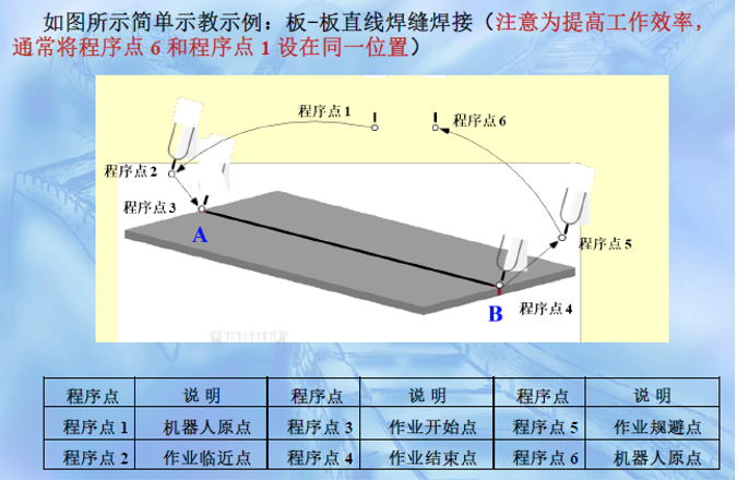
Teaching Steps Example (Focus on Teaching Point Definition and Interpolation Method)
Step 1: Preparation before teaching
Step 2: Create new work program
Step 3: Log program points
Step 4: Set working conditions
Step 5: Check test run
Step 6: Reproduce welding
New Teaching Technologies
Concept of Traction Teaching, Limitations
Hand-in-hand Teaching: Also known as manual traction teaching (also called direct teaching or hand-in-hand teaching). It involves the operator pulling the robot’s end effector equipped with force-torque sensors to perform work on the workpiece, and the robot records the entire teaching trajectory and process parameters in real-time, allowing accurate reproduction of the entire work process based on these online parameters.
Limitations: Accuracy, sensor costs, limitations of teaching workpiece size, etc.
Concept of Remote Operation Teaching, Master-Slave, (understanding) Three Remote Operation Methods, Issues.


(Scan the QR code to view course details)