Linear regression is the foundation of the classic least squares method, Kalman filter, and Wiener filter. It was the first algorithm I encountered during my graduate studies, and I first used it while working on a project for my advisor. After entering the workforce, I found that these algorithms are ubiquitous in engineering. Unfortunately, many colleagues are not familiar with these mathematical algorithms and only use simpler methods like moving average filtering, mean filtering, low-pass, high-pass, band-pass, and notch filters. While these methods are straightforward, they do not perform as well as least squares or Kalman filtering. The key is to apply these algorithms correctly; otherwise, it is better not to use them at all.
In fact, regression algorithms are relative to classification algorithms and are related to the type of target variable y we want to predict. If the target variable y is categorical, such as predicting a user’s gender (male, female), predicting the color of a seasonal flower (red, white, yellow, etc.), or predicting whether someone has lung cancer (yes, no), we need to use classification algorithms to fit the training data and make predictions. Academically, this is typically done using SVM (Support Vector Machine), Particle Swarm Optimization, Neural Networks, etc. However, in embedded development, especially in microcontroller development, these complex algorithms cannot be applied due to their complexity and computational load. Instead, we generally use simpler algorithms like Kalman or least squares methods. Among them, simple linear regression is the easiest to understand and the most widely used algorithm, and it is also a popular introductory algorithm in the current machine learning industry.
Simple Linear Regression
Simple linear regression, as the name suggests, involves one independent variable (which can be the voltage value collected by an ADC, the temperature value collected by a DS18B20, or the light intensity value collected by a photoresistor). Below, we will use the most common voltage collection in our work as an example to predict the linear equation of our voltage collection using simple linear regression, taking the voltage collection system of our IoT development board as an example:
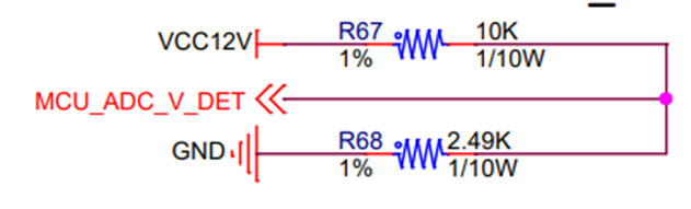
Figure 1: Input Voltage 12V ADC Voltage Collection Circuit
Since the voltage range that the microcontroller can collect is 0-3.3V (it is generally most accurate to collect 60% of the full-scale voltage, which is often considered by hardware engineers when designing circuits), you can see that the hardware circuit uses a voltage divider to reduce the 12V voltage to 1/11, sending this value to the microcontroller’s ADC. The microcontroller collects this voltage value, and multiplying it by 11 gives us the collected voltage value. This is easy to understand because the input voltage is generally fluctuating around 12V, making it easy to backtrack. In practice, we can do this, provided that we do not require high precision in our collection. However, in industrial control or fields requiring high precision measurement and control, we need to use linear regression methods.
Assuming the voltage input range is 4-12V, various errors (integral error, differential error, zero drift, and resistance precision errors in the circuit) can lead to certain inaccuracies in the collected voltage values. To effectively address this issue, we can use the least squares method to predict the linear equation (which involves simple linear regression). Of course, we assume that our system is linear, which our hardware design colleagues should consider from a hardware perspective (circuit impedance matching design, PCB routing, ADC reference voltage, etc.) to ensure that the system is as close to linear as possible. The system cannot be completely linear. If the hardware deviation is too large, the software will be powerless to help. From this perspective, software is an aid to hardware, and algorithms maximize the assistance to hardware.
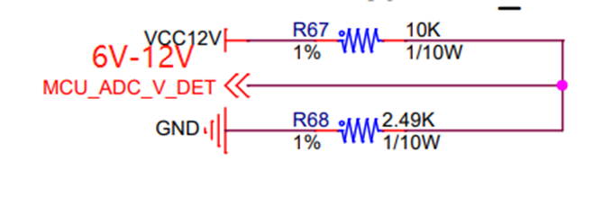 Figure 2: Input Voltage 6V-12V ADC Voltage Collection Circuit
Assuming the linear equation is as shown in (1):
y=β0+β1*x (1)
This is what we commonly refer to as a proportional function. x is the voltage value collected by the ADC, and Y is the input voltage (6V-12V). β0 and β1 are the linear regression coefficients that we aim to predict using mathematical methods.
When we use only one x to predict y, it is called simple linear regression, which involves finding a line to fit the data. For example, if I plot a scatter plot of a set of collected data, y represents the input voltage, and x is the value collected by the microcontroller’s ADC. Linear regression aims to find a line that best fits the data points in the graph.
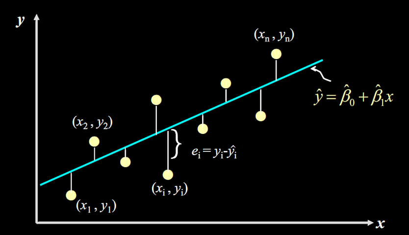
Figure 3: Linear Regression Fitting Graph
Here, the fitting equation we obtain is: y =β^0+β^1*X。Calculating the error ei between the input voltage (yellow discrete points in Figure 3) and the voltage calculated using the fitting function (green line) gives us ei=yi-y^i. We then square this value (to eliminate the negative sign) and calculate it for each point in our data, summing all the e values.
We can quantify the error between the fitted line and the actual data.
In formula form, this is expressed as:
 (2)
(2)
This formula represents the sum of squared residuals, which is our evaluation criterion for the “line”. The smaller the value of this function, the better the line fits our data.
Least Squares Estimation
Now that we know the evaluation criterion for line fitting, our next goal is to predict the values of the coefficients β^0 and β^1.
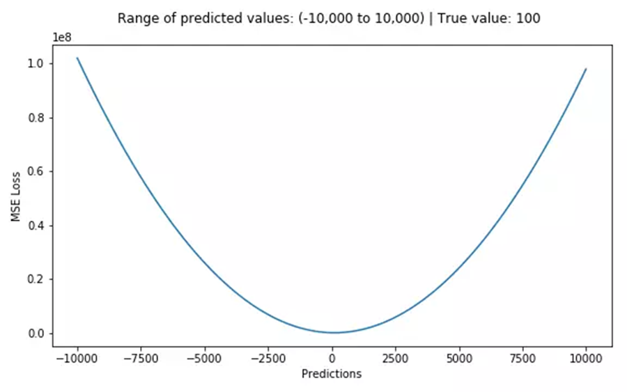
Formula (2) is a quadratic equation, which we know looks something like the following:
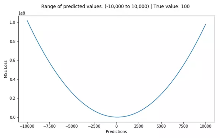
In the above formula, β^0 and β^1 are unknowns, and this quadratic equation has two unknown parameters. The parabola opens upwards, and the point where the derivative is zero is the vertex of the graph, which is referred to as the minimum residual sum, satisfying our evaluation criterion. If you remember your calculus, you know that the derivative is zero when Q reaches its minimum value. Therefore, we take the partial derivatives of β^0 and β^1 and set them to zero:
 (3)
(3)
x_i,y_i(i=1,2,…n) are known (where x_i is collected by the microcontroller and y_i is collected by a high-precision multimeter). By substituting all known values into the above two equations, we can solve for β^0 and β^1. This is the least squares method, where “least squares” refers to squaring the residuals.
The solution obtained from (3) is:
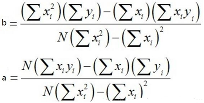 (4)
(4)
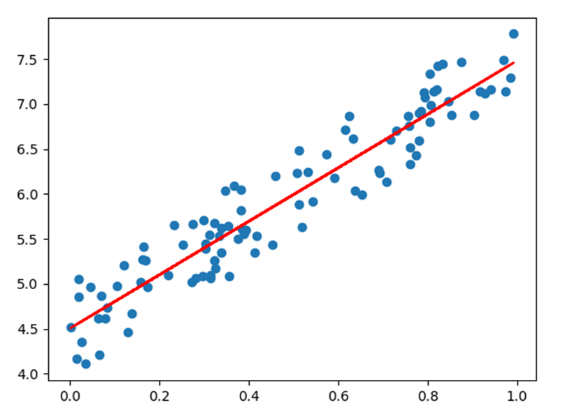
During my time at Feiyu, I used MATLAB to collect some data and performed a simple fitting as shown in the following figure:
What everyone is most concerned about is how to program the microcontroller. Below is the core implementation of this algorithm.
Code Implementation
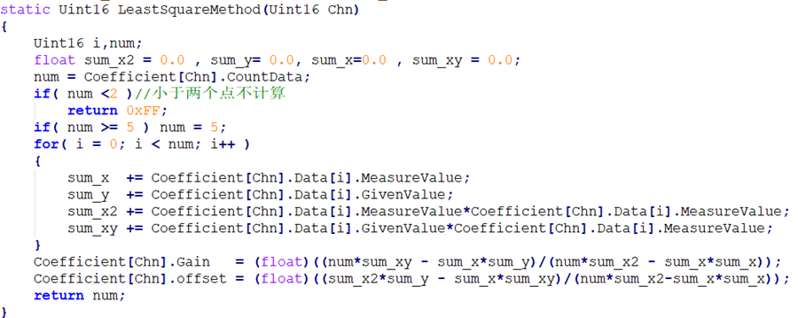
This algorithm can perform least squares optimal estimation for multiple ADC channels, which has been repeatedly verified by Feiyu. Due to limited conditions at home, I will not demonstrate the experimental phenomena. The least squares method is widely used and flexible; it can also estimate measurement errors from sensors.
Source: Feiyu Embedded Newsletter
#Recommended Reading#What connects the joints of a robotic arm?A detailed explanation of robot control systemsHigh-definition dynamic diagrams of mechanical principles, super cool!Understanding the AI knowledge system in one imageSeveral basic circuits for controlling motorsA detailed analysis of the working principles of robots, vivid and illustrative!40 dynamic images to help you intuitively understand electromagnetic fields