"工控有得聊" is a professional information and service platform under the "Mechanical Industry Press" brand, dedicated to helping readers stay updated with cutting-edge information and master core technologies in the fields of electricity, communication, and automation.In electronic circuits, it is necessary to analyze various technical parameters of the circuits produced to determine whether the performance indicators meet the requirements. Multisim 14.0 has rich simulation and analysis functions required for circuits.
Sensitivity Analysis
“Sensitivity” analysis refers to analyzing the impact of changes in the parameters of a certain component in the circuit on the node voltage or branch current of the circuit.
Sensitivity analysis includes DC sensitivity analysis and AC sensitivity analysis. The simulation analysis results of DC sensitivity analysis are displayed in numerical form, while the simulation analysis results of AC sensitivity can be displayed in the form of curves.
To establish a circuit in Multisim 14.0, as shown in Figure 10-19, execute the command “Simulate” → “Analyses and Simulation”. The “Analyses and Simulation” window will pop up, and in the “Active Analysis” option area, select “Sensitivity” to open the “Sensitivity” dialog box, which has four tabs; except for the “Analysis Parameters” tab, the others are the same as “DC Operating Point”. The “Analysis Parameters” tab for sensitivity analysis is shown in Figure 10-20, explained as follows.
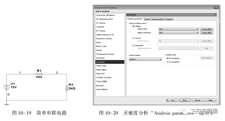
1) Output nodes/currents: Output nodes, which include three radio buttons. The “Voltage” radio button is used to select voltage sensitivity analysis. After selecting this radio button, choose the node to be analyzed from the “Output Node” dropdown list, here select V(2); in the “Output Reference” dropdown list, select the reference node for the output, here select V(0); the “Current” radio button is used to select current sensitivity analysis, similar to the “Voltage” radio button, no selection is made here; the “Expression” radio button is for adding a display form of an expression to the analysis results, no selection is made here for variable expression sensitivity analysis.
2) Output scaling: Used to select the format for output sensitivity, with Absolute (absolute sensitivity) and Relative (relative sensitivity) options, here select “Relative”.
3) Analysis Type: Settings for DC sensitivity analysis or AC sensitivity analysis, here select “DC Sensitivity”.
In the “Output” tab of the sensitivity analysis, set all variables rr1, rr2, vv1 as output nodes. After setting, click the “Run” button, and the sensitivity analysis results are shown in Figure 10-21.
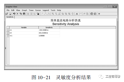
Sensitivity is closely related to error. If the ideal output of the circuit is Y, and X is a parameter in the circuit, then the deviation of the circuit output signal is ΔY/Y = ΔX/X × Z. Here, Z is the sensitivity corresponding to X, equivalent to the value in Figure 10-21. ΔX/X represents the degree of deviation of the component from the nominal value, that is, parameter deviation, which can be expressed as a percentage. In sensitivity analysis, for convenience in understanding the problem, the error of the power supply is generally ignored; in Figure 10-21, the sensitivity of vv1 is 1, because vv1 is the power supply voltage.
Zero-Pole Analysis
The poles of the circuit system transfer function determine whether the system is stable, while the zeros and poles together determine the steady-state performance indicators of the system; therefore, zero-pole analysis of the system transfer function is very necessary. For high-order systems, directly obtaining their zeros and poles is relatively difficult; however, the “Pole Zero” analysis provided by Multisim 14.0 can quickly obtain the system’s zeros and poles.
To establish a simulation circuit in Multisim 14.0 as shown in Figure 10-22, readers can use a signal flow graph combined with Mason’s formula to obtain the system transfer function. Execute the command “Simulate” → “Analyses and Simulation”, and the “Analyses and Simulation” window will pop up; in the “Active Analysis” option area, select “Pole Zero” to open the “Pole Zero” dialog box, whose “Analysis Parameter” tab is shown in Figure 10-23, with the meanings of various parameters as follows.
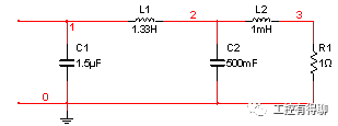
Figure 10-22 Zero-Pole Analysis Simulation Circuit
1) Analysis type: Used to set the type of analysis for zero-pole analysis. There are four selection modes in this option area: Gain Analysis (voltage gain analysis), which is output voltage/input voltage; Impedance Analysis (mutual impedance analysis), which is output voltage/input current; Input Impedance (circuit input impedance); and Output Impedance (circuit output impedance).
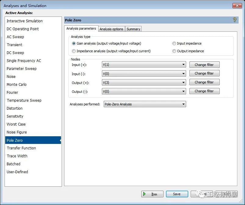
Figure 10-23 Zero-Pole Analysis “Analysis Parameters” Tab
2) Nodes: Used to set the input/output nodes (positive and negative terminals). This option area includes the “Input (+)” dropdown list, which is the positive input terminal; the “Input (-)” dropdown list, which is the negative input terminal (usually grounded, i.e., node 0); the “Output (+)” dropdown list, which is the positive output terminal; and the “Output (-)” dropdown list, which is the negative output terminal (usually grounded, i.e., node 0).
3) Analysis performed: Used to set the analysis object, with three options: Pole Analysis (only finding poles), Zero Analysis (only finding zeros), and Pole-Zero Analysis (finding both zeros and poles).
The settings for Analysis options and Summary are the same as other analysis methods, with default settings. The parameter settings are shown in Figure 10-23.
Click the “Run” button, and the zero-pole analysis results are shown in Figure 10-24, where “Real” represents the real part and “Imaginary” represents the imaginary part. According to the simulation results, it can be seen that the system has no zeros and three poles (approximated), which are -1, -1+0.709j, and -1-0.709j. That is, the system transfer function is: H(s) = 0.5/(s+1)(s+1+0.709j)(s+1-0.709j) = 1/(s³+2s²+2s+1), which is consistent with theoretical analysis.
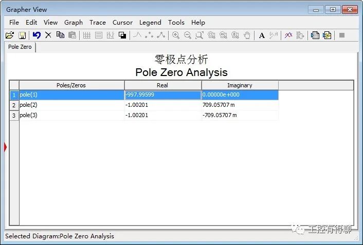
Figure 10-24 Zero-Pole Analysis Results
For more information, you can refer to the book below:
Click on the cover for details
▊《Multisim Circuit Design and Simulation – Based on Multisim 14.0 Platform》
Zhao Quanli, Chief Editor; Wang Xia, Li Huiping, Deputy Editors
-
Comprehensively reflects new developments in the field of Multisim 14 circuit simulation design
-
Includes micro-course videos, focusing on circuit design skills training
This book introduces the knowledge system and application skills of Multisim 14.0 in detail through numerous application examples, including basic operations of Multisim 14.0, analysis, design, and virtual simulation of electronic circuit principles, etc. Each chapter’s application examples are carefully selected and highly targeted, aiming to improve readers’ electronic circuit knowledge while learning Multisim simulation software, achieving a comprehensive understanding and the ability to extrapolate knowledge.The book is divided into 10 chapters, mainly covering three parts:Basic functions and usage of Multisim 14.0;Design, analysis, and simulation of circuits in Multisim 14.0 for circuit analysis, analog circuits, digital circuits, power electronic circuits, and high-frequency electronic circuits;Applications of Multisim 14.0 in MCU circuits.This book can serve as a textbook for teaching and experimental simulation in electrical courses in higher education institutions, as well as a textbook for courses on “Multisim-based Electronic Technology Simulation”, and is also suitable as a textbook for electronic circuit design and simulation for undergraduate, higher vocational, and specialized related majors.