🌠This work includes the program, Chinese comments, references, and a program operation video.🚀Software versions: Matlab 2024b/Matlab 2022a 🌠Program acquisition method
Click the bottom left corner of WeChat to read the original text

 💥Program test results displayThe simulation test results are as follows:
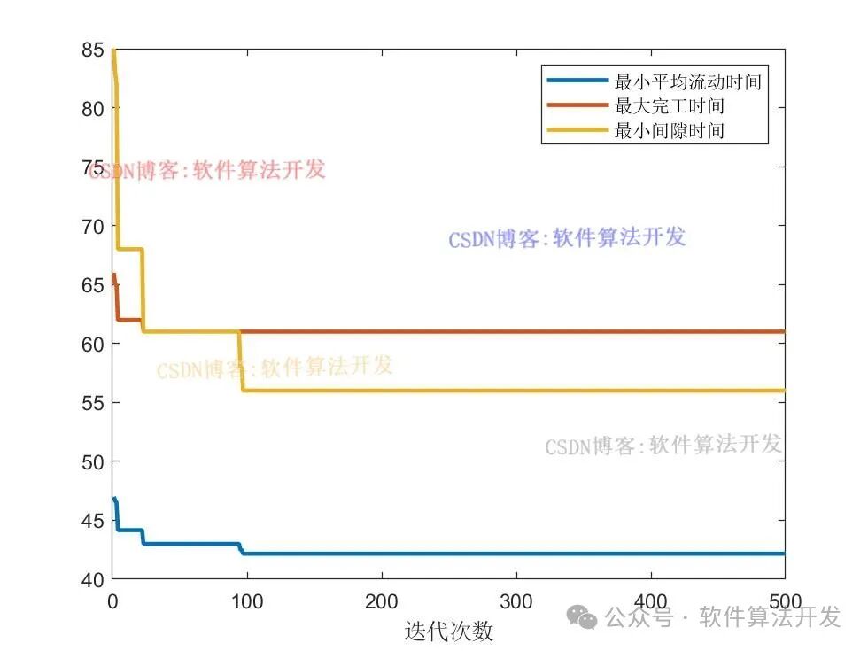
 ✨Algorithm Overview
In the field of modern optimization algorithms, the Simulated Annealing (SA) algorithm stands out with its unique probabilistic mechanism, becoming an important tool for solving complex combinatorial optimization problems, playing a key role in practical applications such as workshop scheduling.
Core Principle of the Algorithm
The design inspiration for the Simulated Annealing algorithm comes from the annealing phenomenon of solids in physics. When a solid is heated to a high temperature, its internal atoms become disordered due to intense thermal motion, deviating from their originally ordered lattice structure. As the temperature gradually decreases, the thermal motion of the atoms weakens, and they continuously attempt to find lower energy positions during their movement, ultimately stabilizing in the state of lowest energy, forming the optimal lattice structure.
At the algorithmic level, SA defines the set of all possible solutions to the problem as the solution space, which corresponds to the state space of the solid. The objective function value of the problem is analogous to energy, and the algorithm continuously explores the solution space by simulating the solid annealing process, attempting to find the optimal solution that minimizes (or maximizes, depending on the specific problem) the objective function value.
The key difference of the SA algorithm from traditional optimization algorithms lies in its unique acceptance criterion. During the search for the optimal solution, this algorithm does not only accept solutions that decrease the objective function value but also accepts those that increase the objective function value with a certain probability. This probability is determined by the Metropolis criterion, and this characteristic endows the algorithm with the ability to escape from local optima traps, allowing for a broader search perspective during exploration, significantly enhancing the likelihood of finding the global optimal solution.
Specific Implementation of Workshop Scheduling Optimization
The workshop scheduling problem essentially seeks to find the optimal combination among numerous possible processing sequences and machine allocation schemes that meet specific objectives (such as minimizing the maximum completion time, reducing total processing costs, etc.), and all these possible combinations constitute the solution space of the workshop scheduling problem.
The SA-based workshop scheduling optimization method deeply integrates the unique advantages of the Simulated Annealing algorithm, continuously exploring the complex solution space by simulating the entire process of solid annealing, effectively avoiding the limitations of local optima, providing an efficient and reliable solution for workshop scheduling problems, and holding significant application value in improving workshop production efficiency and reducing production costs.
 🪐PartProgram
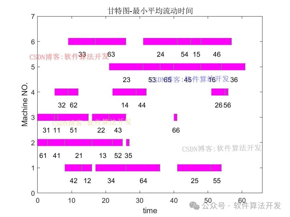
...........................................................................................................................................figure;% Iterate through each element of the optimal particle, decode the time matrix and machine matrix according to the order of the optimal particle, and generate the Gantt chartfor j=1:Ljobs, k=Pbest(j); time(k,counter(k)) = MatTjob(k ,counter(k)) ; machine(k,counter(k))= Matjob(k,counter(k)); % Calculate the start time of the current job process, taking the maximum of the end time of the previous job process and the end time of the previous machine process [rom]=max( s(k), t(machine(k,counter(k))) ); % Update the end time of the previous job process s(k)=rom+time(k,counter(k)); % Update the end time of the previous machine process t(machine(k,counter(k)))=rom+time(k,counter(k)); % Generate the coordinates of the Gantt chart line segments x=[rom t(machine(k,counter(k)))]; y=[machine(k,counter(k)) machine(k,counter(k))]; x1=[t(machine(k,counter(k)))-0.1 t(machine(k,counter(k)))]; y1=[machine(k,counter(k)) machine(k,counter(k))]; % Draw the black line segments of the Gantt chart plot(x,y,'LineWidth',10,'Color','m'); hold on % Draw the white line segments of the Gantt chart (possibly for distinction or decoration) plot(x1,y1,'LineWidth',8,'Color','g'); hold on % Generate an identifier for the current job process a=k*10+counter(k); % Add text annotation to the Gantt chart to display the identifier of the current job process text((rom+t(machine(k,counter(k))))/2-1,machine(k,counter(k))-0.5,num2str(a)) ; hold on % Set the axis range of the Gantt chart, x-axis range from 0 to maximum completion time b plus 5, y-axis range from 0 to 7 axis([0 b+5 0 7]) ; % Increment the position counter by 1, preparing to process the next process counter(k)=counter(k)+1 ;end% Set the x-axis label of the Gantt chart to time (minutes)xlabel('time');% Set the y-axis label of the Gantt chart to machineylabel('Machine NO.');% Set the title of the Gantt chart to Gantt Charttitle('Gantt Chart - Minimum Average Flow Time');102