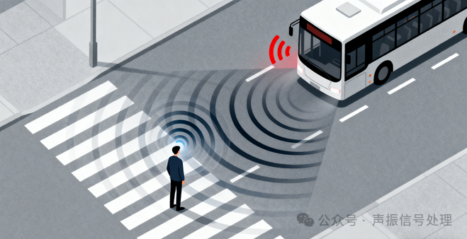
Walking on the road, even in a noisy environment, we can easily identify the direction of a vehicle honking behind us.
In smart home scenarios, we only need to call out the name of AI, and the smart speaker can accurately recognize our voice and respond.
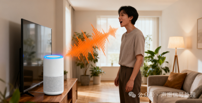
Humans can determine the direction of sound with their two ears, and for smart devices to possess this ability, the key lies in the sound sensor array behind them.
A sound sensor array is not just a simple stack of sensors; its arrangement is like a carefully designed “deployment”, which directly determines how accurately, completely, and stably the device can “hear”.
Today, we will briefly introduce common sound sensor arrays and see how different “formations” enhance the sound source localization capabilities of sensors.
1. First, understand: the underlying logic of sensor sound source localization
No matter what type of array, the core is to help sensors mimic the principle of human “binaural localization”, for example: using the time difference of arrival (Time Difference of Arrival, TDOA) at different sensors.
For humans, when sound comes from the left, the left ear receives the sound before the right ear (TDOA), and the brain instantly locks onto the direction of the sound by analyzing this time difference.
The sound sensor array captures more dimensions of time and intensity differences through multiple sensors arranged in a specific “formation”.
The more sensors there are and the more reasonable the “formation” is, the richer the sound difference information collected, and naturally, the better the device’s sound source localization capability. In simple terms: the “formation” of the sensor array is the “hardware core” of sound source localization, directly affecting the accuracy, range, and reliability of the localization.
2. In-depth analysis of different sensor arrays: each has its strengths and weaknesses, suitable for different scenarios
The differences in “formation” among different arrays lead to varying focuses in sensor sound source localization. Below, we will analyze the characteristics of common linear, circular, cross, and random sensor arrays one by one.
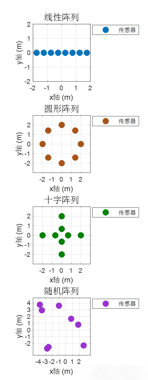
1. Linear array: “One-dimensional localization vanguard”, a simple and practical entry-level “formation”
Characteristics: All sensors are arranged in a straight line. This layout is very simple and low-cost, making it the first choice for many entry-level devices.
Impact on sound source localization:
Advantages: In the linear dimension, its accuracy is acceptable. It is very easy to integrate into narrow devices like smartphones and smart speakers.
Disadvantages: This is the most limited performance formation. It is essentially a one-dimensional system, and the insufficient information dimension leads to its inability to reliably calculate the two-dimensional position of the sound source. There is usually a “fuzzy axis”, making it difficult to distinguish sound sources in front of and behind the array, resulting in significant localization errors.
Typical applications:
Conference microphones: Capturing speakers on both sides of the conference table.

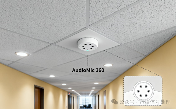
2. Circular array: “Omnidirectional localization guardian”,360° no blind spots“formation”
Characteristics: Multiple sound sensors are evenly distributed along the same circumference.
Impact on sound source localization:
Advantages: It has the potential for omnidirectional localization, with uniform performance in all directions, theoretically providing very high localization accuracy.
Disadvantages: Its performance heavily depends on the balance between the number of sensors and the size (aperture) of the array. If the array is too small, the localization accuracy is low; if the array is too large, it poses significant computational challenges, which can lead to algorithm failure and decreased accuracy.
Typical applications:
Security monitoring:360° monitoring of unusual sounds in corridors and halls, such as footsteps and lock-picking sounds.
3. Cross array: “Two-dimensional localization expert”, balancing horizontal and vertical “formation”
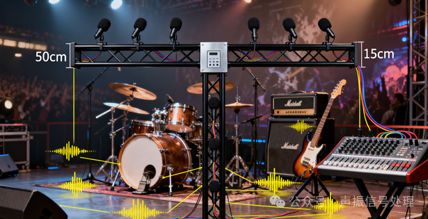
Characteristics: Sound sensors are arranged along two mutually perpendicular lines, forming a “cross” shape.
Impact on sound source localization:
Advantages: It can capture information in two dimensions simultaneously, effectively avoiding the localization ambiguity problem of linear arrays. Its greatest advantage is robustness; as the number of sensors increases, its localization performance typically improves in a stable and predictable manner, making it an excellent choice for balancing performance and complexity.
Disadvantages: The accuracy in the diagonal direction of the cross may be slightly lower than in the main axis direction. It requires at least 4 sensors, making it more expensive than linear arrays.
Typical applications:
Stage monitoring equipment: Accurately capturing sounds from instruments at different heights on stage, such as drums on the ground and guitars above.
4. Random array: “Interference-resistant warrior”, suitable for complex environments“formation”
Characteristics: Sensors are irregularly distributed within an area. This is often a last resort when internal space constraints exist in devices.
Impact on sound source localization:
Advantages: Random distribution often breaks the inherent symmetry of regular arrays, thus avoiding severe localization ambiguity in certain directions. As long as there are enough sensors, its average performance is often quite good.
Disadvantages: Performance is unpredictable and fluctuates greatly. Each deployment layout is random, which may perform well this time but poorly the next. It cannot guarantee a consistent user experience.
Typical applications:
Low-cost children’s smart toys: Meeting simple voice interaction localization needs.
3. Besides the array “formation”, these factors are also crucial
Choosing the right sensor array “formation” does not guarantee perfect sound source localization. The following factors will also directly affect the localization effect:
1. Trade-off between the number of sensors and the array aperture:
The more “forces” there are, the better they can theoretically hear. But more importantly, how the sensors are distributed matters. A well-designed small array may outperform a large and sparse array. The physical size (aperture) of the array must match the expected distance to the sound source.
2. Algorithms are the brain:
The raw time difference signals captured by the hardware require powerful signal processing algorithms to resolve them into location information. The algorithms need to overcome interference from noise, echoes, and multipath effects.
3. Environmental interference:
Noisy and echo-prone environments are “localization killers”. Advanced algorithms must include anti-interference modules to maintain stability in real-world scenarios.
Key point:
Hands-on practice
4. The research team explores the localization effects of different arrays
Assuming there is a point sound source emitting sound signals on a plane, we will compare the localization effects using different sensor arrays to receive sound wave signals.
The following diagram shows the planar distribution of four different sensor arrays:
The research team used the time difference of arrival TDOA localization theory to perform sound source localization under different formations, determining the position of the sound source by solving a set of hyperbolic equations.
The Euclidean distance from the sound source to the ith sensor di is:

The time required for sound to travel from the sound source to the ith sensor ti is:

where c is the speed of sound.
Taking the first sensor as a reference, the time difference of arrival at the ith microphone τi1 is:
From this, we obtain the distance difference equation, which defines a hyperbola with m1 and mi as foci, with the sound source located on this curve:
 The position of the sound source was calculated using the nonlinear least squares method as follows: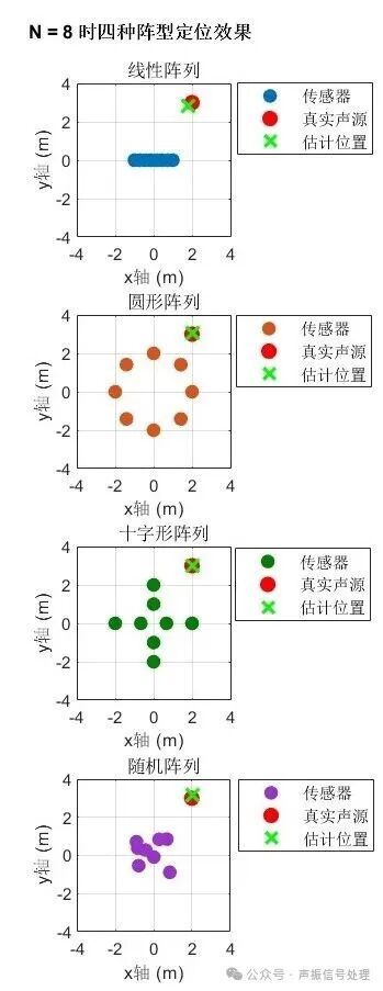
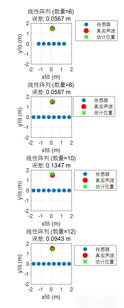
Exploring the localization effects of different sensor numbers:
The localization effect of the linear array is as follows:
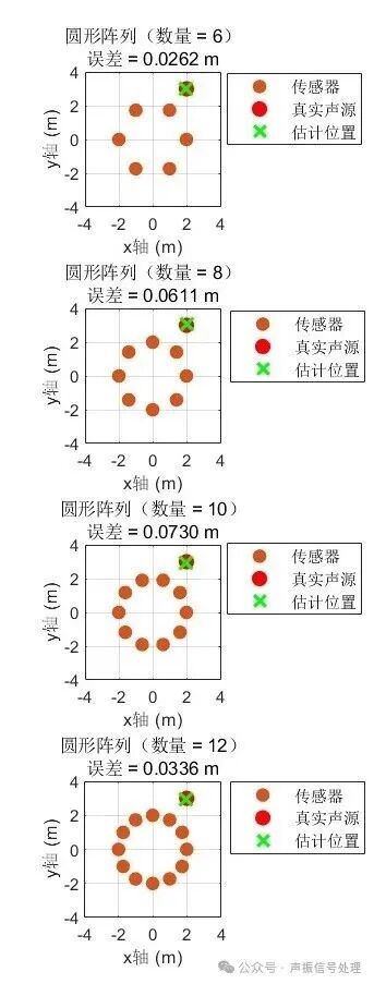
The localization effect of the circular array is shown in the figure:
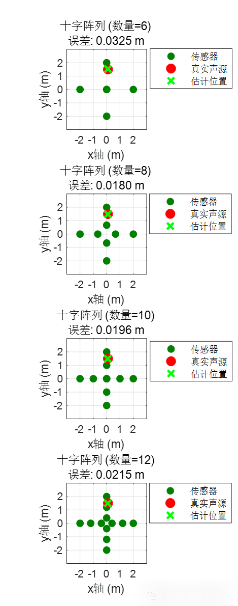
The localization effect of the cross array is shown in the figure:
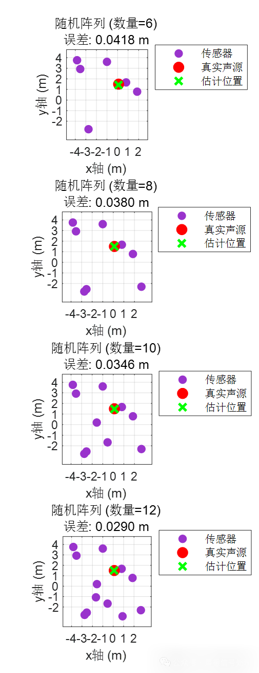
The localization effect of the random array is shown in the figure:
The comprehensive localization effects of different array formations are influenced by the number of sensors as shown in the figure below:
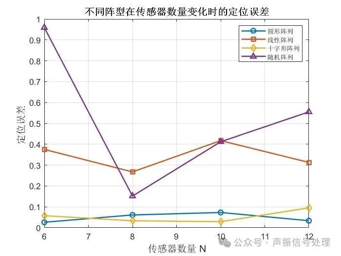
Analysis of this:
The linear array can only constrain one direction well, and there may be errors in the vertical direction. When the number of elements is large, the overall constraint increases, and the error tends to stabilize and decrease.
The circular array performs stably, but there are fluctuations under different sensor numbers, as the circular array is prone to mirror convergence under this simulation and optimization scheme.
The cross array shows a stable improvement trend as the number of sensors increases, as it provides two-dimensional spatial resolution, avoiding the front-and-back ambiguity problem of linear arrays.
The random array avoids localization ambiguity zones by breaking the regular structure, and while it may perform well on average, it cannot guarantee reliability in practical applications unless extensive layout optimization is performed.
5. Conclusion: Choose the “formation” as needed to make sensors “hear in all directions” more efficiently
The impact of different array “formations” on sensor sound source localization is essentially a balance between “localization capability” and “cost, complexity”. In sound source localization technology using sensor arrays, the most suitable and accurate array formation should be selected according to needs to achieve precise localization.
With the development of technology, perhaps in the future, there will be “adaptive arrays”— through AI algorithms, allowing simple “formations” to achieve complex localization effects. Next time you wake up a device with a voice assistant, pay attention to the sound sensor array behind it, and consider which “formation” it is using to achieve precise sound source localization?
Content sourced from the research team Chen Yingying Master’s