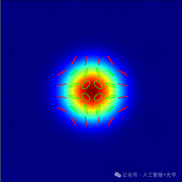
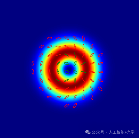
IntroductionIn the study of Vector Optical Fields, the simple distribution of Intensity often obscures the physical essence. How can we intuitively display the complex evolution of polarization states across the cross-section of a beam? How can we use color to distinguish between left-handed and right-handed circular polarization? In this issue, we will learn how to create scientific illustrations of “Intensity background + Polarization ellipse array”.🌄 Using MATLAB to visualize vector vortex light with polarization states
clc; clear; close all;%% 1. Parameter settingsN = 300; L = 1.5e-3; x = linspace(-L, L, N);y = linspace(-L, L, N);[X, Y] = meshgrid(x, y);[Phi, R] = cart2pol(X, Y);%% 2. Generate complex vector light field (Poincaré Beam)% Use superposition of circularly polarized light with different topological charges to produce spatially varying polarization statesw0 = L/3; % Define two orthogonal circular polarization bases (Right Circular & Left Circular)l1 = 0; l2 = 2; % Amplitude envelopeEnv = exp(-R.^2/w0^2);% Construct right and left circular polarization components (ER and EL)ER = Env .* exp(1i * l1 * Phi); % Right-handed componentEL = Env .* (R/w0) .* exp(1i * l2 * Phi); % Left-handed component % Convert circular polarization basis to Cartesian coordinates (Ex, Ey) for plottingEx = (ER + EL) / sqrt(2);Ey = -1i * (ER - EL) / sqrt(2);% Calculate total intensityIntensity = abs(Ex).^2 + abs(Ey).^2;S3 = 2 * imag(conj(Ex) .* Ey);%% 3. Plot background intensityfigure('Color', 'w', 'Position', [100, 100, 700, 600]);% Plot intensity map with deep blue backgroundh = pcolor(X*1e3, Y*1e3, Intensity); set(h, 'EdgeColor', 'none');shading interp;colormap(parula); % or use jet / hotaxis equal; axis tight;set(gca, 'Color', [0 0 0.1]); % Dark backgroundxlabel('x (mm)'); ylabel('y (mm)');title('Vector Optical Field Polarization (Red: Right-handed, Green: Left-handed)');hold on;%% 4. Plot polarization ellipsestep = 20; % Sampling intervalscale = 0.08; % Ellipse scaling factorthreshold_I = max(Intensity(:)) * 0.1; % Intensity threshold, do not plot where too dimt = linspace(0, 2*pi, 30); % Time parameter for drawing ellipse trajectoriesfor r = 1:step:N for c = 1:step:N I_loc = Intensity(r, c); if I_loc < threshold_I continue; % Do not plot if light is too weak end % Get S3 value and electric field at this point S3_loc = S3(r, c); Ex_loc = Ex(r, c); Ey_loc = Ey(r, c); % Calculate ellipse trajectory ex_trace = real(Ex_loc * exp(1i * t)); ey_trace = real(Ey_loc * exp(1i * t)); % Normalize size (to make the ellipse look clear and uniform) max_amp = max(sqrt(ex_trace.^2 + ey_trace.^2)); if max_amp > 0 ex_trace = ex_trace / max_amp * scale; ey_trace = ey_trace / max_amp * scale; end if S3_loc > 0 col = [1, 0, 0]; % Red else col = [0, 1, 0]; % Green end % Transform coordinates to grid position px = X(r, c)*1e3 + ex_trace; py = Y(r, c)*1e3 + ey_trace; % Draw line plot(px, py, 'Color', col, 'LineWidth', 1.5); endendset(gca, 'FontSize', 12, 'LineWidth', 1.2);xlim([-L*1e3 L*1e3]);ylim([-L*1e3 L*1e3]);box on;hold off;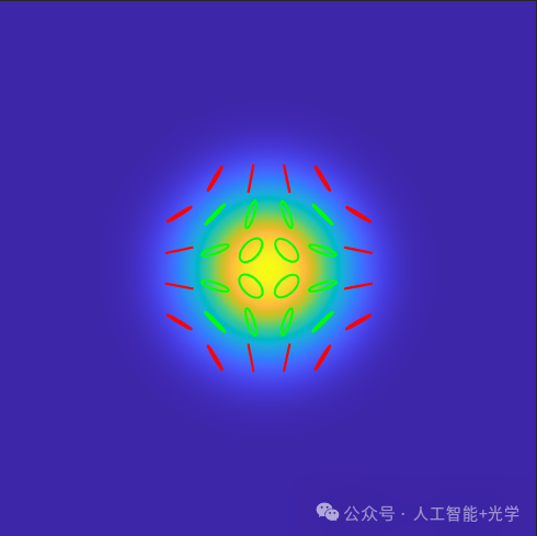
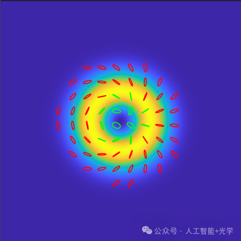 🌄 Using Python to visualize vector vortex light with polarization states
import numpy as npimport matplotlib.pyplot as plt# %% 1. Parameter settingsN = 300 L = 1.5e-3 x = np.linspace(-L, L, N)y = np.linspace(-L, L, N)X, Y = np.meshgrid(x, y)Phi = np.arctan2(Y, X) R = np.hypot(X, Y) # %% 2. Vector light field (Poincaré Beam)w0 = L / 3l1 = 0l2 = 2Env = np.exp(-R**2 / w0**2)ER = Env * np.exp(1j * l1 * Phi) EL = Env * (R/w0) * np.exp(1j * l2 * Phi) Ex = (ER + EL) / np.sqrt(2)Ey = -1j * (ER - EL) / np.sqrt(2)Intensity = np.abs(Ex)**2 + np.abs(Ey)**2S3 = 2 * np.imag(np.conj(Ex) * Ey)# %% 3. Plot background intensityfig, ax = plt.subplots(figsize=(8, 7), dpi=100)c = ax.pcolormesh(X*1e3, Y*1e3, Intensity, cmap='jet', shading='gouraud')ax.set_facecolor((0, 0, 0.1)) ax.set_aspect('equal')ax.set_xlabel('x (mm)', fontsize=12)ax.set_ylabel('y (mm)', fontsize=12)ax.set_title('Vector Optical Field Polarization (Red: Right, Green: Left)', fontsize=13)ax.set_xlim([-L*1e3, L*1e3])ax.set_ylim([-L*1e3, L*1e3])# %% 4. Plot polarization ellipsestep = 20 scale = 0.08 threshold_I = np.max(Intensity) * 0.1 t = np.linspace(0, 2*np.pi, 30) for r in range(0, N, step): for c in range(0, N, step): I_loc = Intensity[r, c] if I_loc < threshold_I: continue S3_loc = S3[r, c] Ex_loc = Ex[r, c] Ey_loc = Ey[r, c] # Calculate ellipse trajectory (real part) ex_trace = np.real(Ex_loc * np.exp(1j * t)) ey_trace = np.real(Ey_loc * np.exp(1j * t)) # Normalize size max_amp = np.max(np.sqrt(ex_trace**2 + ey_trace**2)) if max_amp > 0: ex_trace = (ex_trace / max_amp) * scale ey_trace = (ey_trace / max_amp) * scale # Determine color color = 'red' if S3_loc > 0 else 'lime' # Use lime for a brighter green # Transform coordinates and plot px = X[r, c]*1e3 + ex_trace py = Y[r, c]*1e3 + ey_trace ax.plot(px, py, color=color, linewidth=1.5)plt.tight_layout()plt.show()