Introduction
Proteus is a widely used software for circuit design, testing, and debugging. The Proteus product suite includes tools for describing circuits, simulating circuits, and designing and auto-routing printed circuit boards. Proteus is an electronic circuit design program that combines professional features with ease of use, suitable for both educational purposes and the industrial production of complex electronic devices.
Proteus is an end-to-end design platform that combines two core programs: ISIS, a schematic design and simulation module that allows professionals to optimize their designs, minimize errors, and reduce iterations during the development process; and ARES, a printed circuit board (PCB) layout design software.
The program includes a set of virtual instruments for measurement: voltmeters, ammeters, four-channel oscilloscopes, logic analyzers, signal generators, digital pattern generators, power meters, and virtual terminals.
Proteus virtual instruments are software models of control and measurement devices that correspond to real devices. Using virtual instruments in Proteus is a simple and intuitive way to interact with circuits, and when testing or creating electronic devices, it operates almost identically to traditional methods. It is the easiest way to verify the behavior of developed circuits.
By adjusting the devices, you can:
- Change the instrument scale according to the measurement range;
- Set the operating mode of the device;
- Set the type of input effects for the circuit (DC and harmonic currents and voltages, triangular waves, and rectangular pulse waves).
The graphical capabilities of the program allow you to:
- Simultaneously observe several curves on the graph;
- Display curves in different colors on the graph;
- Transfer data to a graphic editor for necessary transformations and printing.
All Proteus instruments operate (connected to the circuit and used) exactly the same as their real-world counterparts. To add a virtual instrument to the program’s workspace, click its name in the “Instruments“ panel (by default, this panel is located on the left side of the program and contains a list of available virtual instruments), and then use the mouse to place it at the desired location on the circuit. Click the ISIS editor’s left toolbar on the “Instrument Mode“ button to open the “Instruments“ panel. After the circuit simulation starts, the instrument’s front panel will open. You can configure the necessary settings just like on the panel of a real instrument. Connecting the virtual instrument to circuit components is the same as with other circuit components. Multiple instruments can be used in each circuit, including multiple copies of the same instrument. Each copy needs to be configured and connected separately. Next, we will detail how to use each virtual instrument in Proteus.
Using Virtual Instruments in Proteus
Ammeter
An ammeter is an instrument used to measure the strength of DC and AC currents in a circuit. Its reading depends on the amount of current flowing through it, so its resistance should be as low as possible relative to the load resistance.
In Proteus, current measurement uses two virtual ammeters: a DC ammeter and an AC ammeter. The DC ammeter is used only to measure the DC component of a signal. If you need to measure the root mean square value of a signal, use the AC ammeter. The ammeter parameters are configured in the “Edit Component“ window (Figure 1) by double-clicking the device icon to open this window.
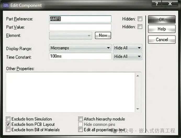
Figure 1. Setting ammeter parameters in the “Edit Component“ window
Using the virtual ammeter is very simple. For example, to measure the current in a branch between two nodes in the circuit, just connect the virtual ammeter in series to the circuit, just like connecting a real ammeter. If you need to measure the current at another node in the circuit simultaneously, connect a second ammeter in series to the circuit. The measurement results will be displayed in the “Results Window“ of the ammeter icon. Figure 2 shows an example of connecting two ammeters to the circuit.
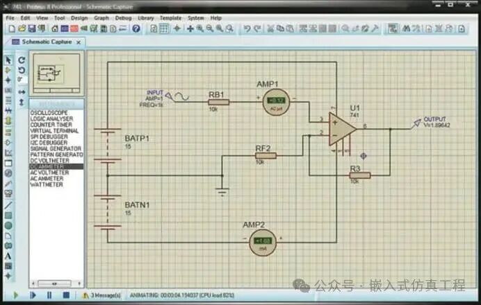
Figure 2. Connecting two ammeters to the circuit
Four-Channel Oscilloscope
An oscilloscope can measure the following electrical signal parameters: voltage, current, frequency, and phase shift angle. This device allows you to observe the waveform of a signal as it changes over time. A dual-channel oscilloscope is the most commonly used, but many engineers choose four-channel models because they are designed to address a wider range of issues. In Proteus, the four-channel oscilloscope has four signal inputs (channels A, B, C and D), allowing it to display the waveforms of four signals simultaneously. The oscilloscope is grounded by default, so there is no ground pin. There are also no external synchronization pins. The icon of the four-channel oscilloscope on the schematic and its front panel are shown in Figure 3 . After running the circuit simulation, the device’s front panel will open. This icon is used to connect the device to the circuit, while the front panel is used to configure the device and view the waveforms of the signals being analyzed. The left side of the front panel of the four-channel oscilloscope has a graphical display area for visualizing waveforms, specifically, the vertical axis displays voltage, and the horizontal axis displays time. The device is also equipped with cursors for time-domain measurements, which can be moved using the left mouse button. To add a cursor, click the oscilloscope control panel “Trigger“ window’s “Cursor“ button. To place a cursor, click the left mouse button in the chart area as many times as needed. To clear the cursor display, right-click and select “Delete Cursor“ to remove a single cursor, or select“Clear All Cursors“ to remove all added cursors. Clicking the “Trigger“ window’s “Cursor“ button again will clear the cursor display and exit cursor placement mode. The time and voltage values of the measured point (the intersection of the cursor and the sine wave) will be displayed before and after moving the cursor.
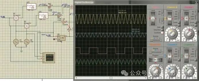
Figure 3. Connecting the four-channel oscilloscope to the circuit and its front panel
The oscilloscope’s control panel is located on the right side of the front panel and is used to configure the display of the measured signal. Let’s take a closer look at this panel.
The control panel contains six setting windows:
- Trigger (Synchronization)
- Channel A (Channel A);
- C Channel (Channel C);
- B Channel (Channel B);
- D Channel (Channel D);
- Horizontal (Scan).
Let’s take a look at the “Channel A” window. At the bottom, there is a knob for setting the Y axis scale value (voltage per division). The starting point of the signal output on the Y axis is specified by the “Position“ field. The value of this field can be positive or negative. Choosing a positive value will move the starting point up along the Y axis, while choosing a negative value will move the starting point down. The working mode can be selected by sliding the slider, with four positions available: AC, DC, GND and OFF. In AC mode, only the AC component of the signal is displayed. In DC mode, the sum of the AC and DC components of the signal is displayed. If the GND position is selected, the input channel is grounded, and a straight line will be displayed at the initial position of the Y axis on the graphical display. Setting the slider to the OFF position will disable the display of the signal on the screen.“Channel A” window also contains two buttons:
- Invert — Sets the oscilloscope to reverse operation mode, where the signal is inverted relative to the zero position;
- A+B — Sets the total signal of channels A and B to be displayed on the graphical display.
Channel C, Channel B and Channel D windows have interfaces similar to the previously discussed Channel A window, except that the Channel C window does not have the A+B button, but instead has the C+D button for setting the display mode of the total signals of channels C and D on the graphical display. The Channel B and Channel D windows do not have such buttons at all.
Let’s take a look at the “Horizontal“ window. At the bottom of the window, there is a control handle for setting the X axis division value. The starting point of the signal output on the X axis is specified in the “Position
field. The value of this field can also be positive or negative. Selecting a positive value will move the starting point of the signal output to the right, while selecting a negative value will move the starting point to the left. The scan mode is selected in the “Source“ field by moving the slider to one of the following positions: ˄, A, B, C, D. Selecting the ˄ mode (signal along the Y axis/time axis) will display the signals of channels A, B, C, D on the Y axis of the graphical display, while the X axis will be the time axis. The modes A, B, C, D are used to observe Lissajous figures (Figure 4). Selecting this mode helps to study the phase of the signals.
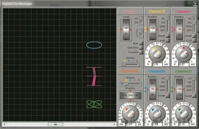
Figure 4. Lissajous figure on the four-channel oscilloscope display
Trigger window is located at the upper left corner of the oscilloscope control panel. The selection of the trigger channel is made in the “Source“ field by moving the slider to one of the positions: A, B, C or D . You can also select the triggering method for the trigger signal by moving the slider to the corresponding position in the respective field, either edge-triggered or falling edge-triggered.
Trigger window has buttons for selecting synchronization modes:
One-Shot (One-Shot) — A mode that waits for a synchronization signal. This mode allows recording a single signal;
Auto (Automatic) — When the oscilloscope is connected to the circuit and the circuit simulation is turned on, the oscilloscope will automatically start.
The operation results of the four-channel oscilloscope are displayed on the graphical display located on the left side of the device’s front panel, in the form of four curves, each representing one of the four input signals received from inputs A, B, C, D.
Signal Generator
In Proteus, the signal generator is used to generate sine, triangular, sawtooth, or square wave test signals with an amplitude range of 0 to 12 V and a frequency range of 0 to 12 MHz. It can input these signals into analog circuits. The device has four terminals: positive (+), negative (-), and amplitude (AM) and frequency (FM) modulation inputs. The positive terminal is used to connect the signal generator to the circuit, while the negative terminal is used to ground the device.
Figure 5 shows the front panel of the signal generator, its icon in the circuit diagram, and an example of its connection to the circuit.
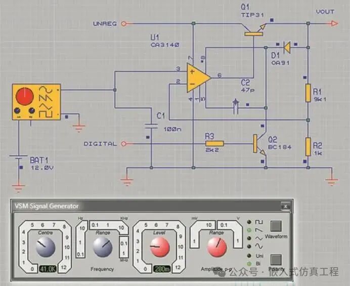
Figure 5. Front panel of the signal generator, its icon, and an example of connection to the circuit
The front panel of the signal generator is used for inputting device settings. Let’s take a closer look at this panel. The right side contains waveform indicators. Use the “Waveform“ button located at the top right of the panel to select the waveform, pressing the button repeatedly until the indicator shows the desired waveform. These indicators are unlabeled, but their functions are intuitive, as each indicator is accompanied by the waveform of the output signal generated. The corresponding “Frequency“ and “Amplitude“ peak switches can be used to set the frequency and amplitude of the generated signal. The Polarity button is used to set the polarity of the signal: unipolar or bipolar.
To visually demonstrate the operation of this device, we will use a virtual oscilloscope and connect it to the positive terminal of the signal generator. We will set the signal generator to produce a sine wave with a frequency of 1.9 kHz. The generated signal is displayed on the oscilloscope screen (Figure 6). As shown in the figure, the amplitude and waveform of the signal correspond to the settings on the signal generator panel — 2.8 V, sine wave.
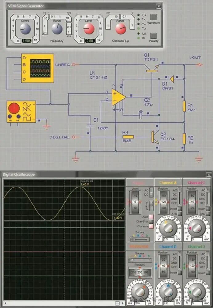
Figure 6. Generating a sine signal with the signal generator and its display on the oscilloscope screen
The signal generator supports amplitude modulation and frequency modulation of the output signal. The amplitude modulation input and frequency modulation input have the following features:
- The modulation input gain can be adjusted using the Frequency and Amplitude Peak switches on the front panel of the signal generator. For example, if the frequency setting on the front panel is 2 kHz, then a 2 V level at the frequency modulation input will produce an output frequency of 4 kHz.
- The input modulation voltage is limited to 12V;
- The modulation input has infinite input impedance.
Voltmeter
A voltmeter is an instrument used to measure electromotive force or voltage in a circuit.
Proteus supports voltage measurement using two types of virtual voltmeters: a DC voltmeter and an AC voltmeter. The DC voltmeter is used only to measure the DC component of a signal. If you need to measure AC voltage, use the AC voltmeter. The voltmeter parameters are set in the “Edit Component“ window (Figure 7) by double-clicking the device icon to open this window. By default, the voltmeter resistance is set to 100 megaohms, but it can be changed by entering the desired value in the “Load Resistance“ field in the “Edit Component“ window. In the “Display Range“ menu, you can set the voltage unit by selecting from the dropdown list: “Volts“, “Millivolts“ or “Microvolts“.
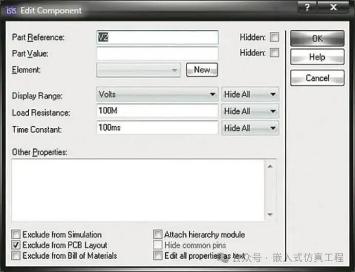
Figure 7. Setting voltmeter parameters in the “Edit Component“ window
Operating this device is very simple. For example, to measure the voltage across any component in the circuit, just connect the virtual voltmeter in parallel with the load being measured, just like using a real voltmeter. The voltmeter can display intermediate values until the final voltage is determined. If you need to measure the voltage of another circuit component simultaneously, connect a second voltmeter in the circuit.
The measurement results are displayed in the “Results Window“ of the voltmeter icon. Figure 8 shows an example of connecting two voltmeters to the circuit.
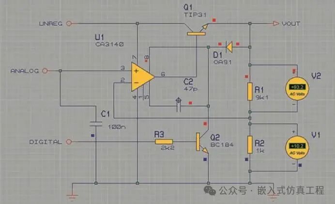
Figure 8. Connecting two voltmeters to the circuit
Wattmeter
A wattmeter is a specialized device for measuring active power. The measurement results are displayed in watts. Figure 9 shows how the wattmeter is connected to the circuit.
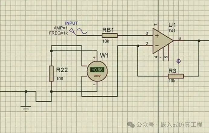
Figure 9. Connecting the wattmeter to the circuit
The measurement results, especially the average power, will be displayed in the “Results Window“ of the wattmeter icon. This device is very simple to operate. To determine the power on the load, connect the upper and lower input terminals of the wattmeter in parallel with the load, and connect the input terminals on both sides in series. The results will be displayed in the “Results Window“. The example shown in Figure 9 demonstrates how to determine the power consumption of the resistor R22 in the shown circuit fragment. The wattmeter parameters are configured in the “Edit Component“
window (Figure 10) by double-clicking the device icon to open this window.
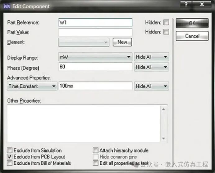
Figure 10. Setting wattmeter parameters in the “Edit Component“ window
Logic Analyzer
A logic analyzer is designed to monitor the state of logic elements in digital electronic devices during the development of large systems and is used for troubleshooting. To capture the signals of the circuit being tested, the logic analyzer is equipped with 16 pins and four 8-bit buses. Figure 11 shows the appearance of the logic analyzer, its connection to the circuit, and its front panel. When the circuit simulation is running, the front panel will automatically open. Let’s take a closer look. The left side of the panel has 16 switches corresponding to 16 signal capture channels: A0–A15.
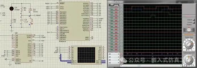
Figure 11. Appearance of the logic analyzer, its connection to the circuit, and its front panel
The next column displays the input names of the logic analyzer. After running the circuit simulation, the device reads the input values from its terminals and displays the result data in the form of rectangular pulses on the front panel’s time-domain clock graph. The lower part of the time-domain graph shows the signals received from inputs B0[0–7] to B3[0–7] . The device is also equipped with cursors for performing time-domain measurements, which can be moved using the left mouse button.
The right side of the device’s front panel has a control panel with two windows:
- Trigger (Synchronization)
- Horizontal (Scan).
Cursors are managed in the “Trigger“ window. The “Cursor“ button allows you to activate or deactivate the cursor. To place a cursor, click the “Cursor“ button, then click the left mouse button in the chart area as many times as needed to place the cursor. To clear the cursor display, right-click and select “Delete Cursor“ to remove a single cursor, or select“Clear All Cursors“ to remove all added cursors. You can click the “Trigger“ window’s “Cursor“ button again to clear the cursor display and exit cursor placement mode.
The logic analyzer processes the digital input data written to the capture buffer in sequence. The data capture process is initiated by clicking the Capture button in the Trigger window. After a brief delay, once the trigger condition is met, the capture process stops, and the button changes color during and after recording. The contents of the capture buffer are displayed on the screen. The Horizontal window contains two knobs: “Display Scale“ and “Capture Resolution“. The former is used to scale the chart display, while the latter is used to adjust the resolution.
The color scheme of the logic analyzer’s graphical display is configured in the “Color Settings“ window (Figure 12) by right-clicking the graphical display area and selecting “Color Settings“ from the context menu. This window specifies the color scheme for displaying (“Display“ column) and printing (“Printer“ column) the following graphical display elements:
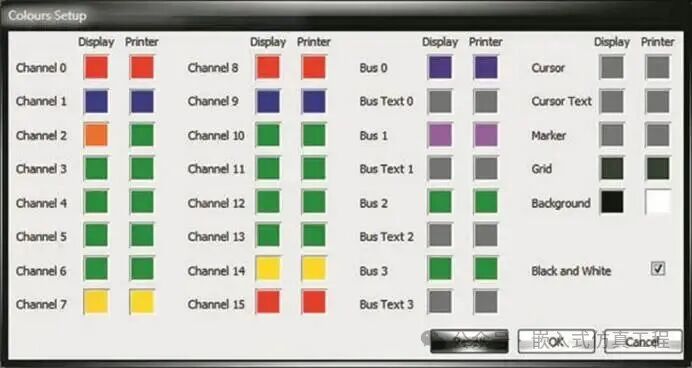
Figure 12. Color settings window
- Display signals (Channel 0 – Channel 15, Bus 0 – Bus 3);
- Text descriptions (Bus text 0 – Bus text 0 – 3, Cursor text);
- Cursor (Cursor);
- Marker (Marker);
- Grid (Grid);
- Background of the graphical display (Background).
The set colors will be displayed in the form of icons next to the names of the graphical display elements. To set a color, left-click the desired icon, select a color from the opened color palette (Figure 13), and then click “OK“.
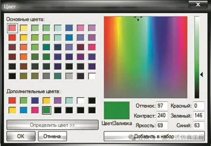
Figure 13. Color window
You can use the “Color Settings“ window’s “Reset button to reset the color scheme to default values. Checking the “Black and White“ checkbox will set the printing color scheme of the graphical display image to black and white. After configuring all color scheme settings, click “OK“.
You can print a snapshot of the logic analyzer’s graphical display by right-clicking the display area and then left-clicking “Print“ from the context menu. This will open the “Print“ window (Figure 14). In the “Select Printer“ field, select the active printer or print to file (Microsoft Office Document Image Writer), and then click “Print“. If you choose to print to file, the “Save Document“ window will open. In this window, you can specify the file name, type, and location on the computer disk, and then click “Save“. The chart will be saved in *.tiff file format to the specified folder (Figure 15).
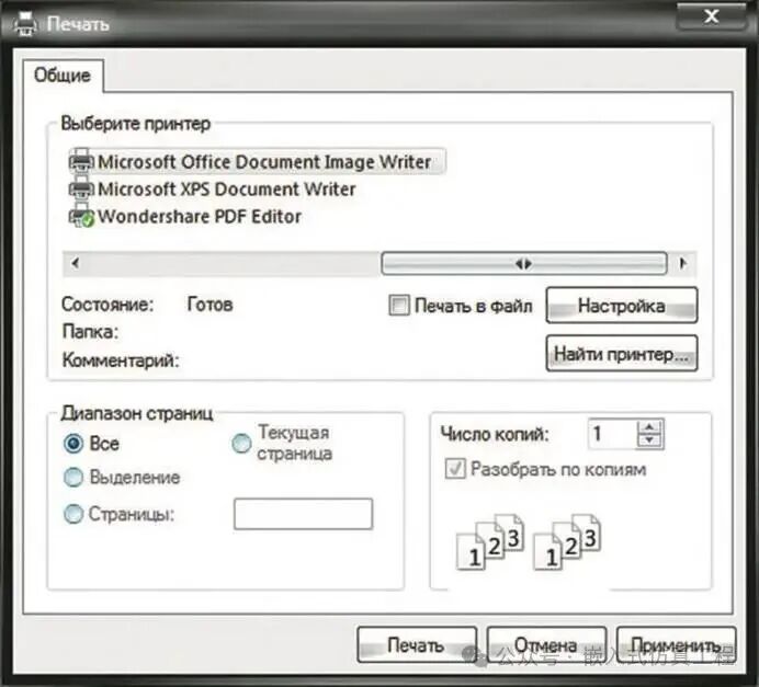
Figure 14. Print window
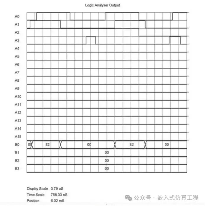
Figure 15. Result of printing a snapshot of the logic analyzer’s graphical display to a file
The operation results of the logic analyzer are displayed in the form of graphs on the graphical display, representing the input signals received from its input terminals.
Conclusion
Proteus offers a wide variety of virtual instruments for analyzing circuits developed in its environment, assigning input signals to circuits, measuring various physical quantities, and plotting graphs. The operating modes and settings of all instruments can be changed. As you can see, the display forms of all instruments are very similar to real instruments, making them very convenient to use.
Proteus is a convenient and practical circuit simulation tool for studying the operation of circuits. The simulation results can be printed or imported for further processing.
Before running circuit simulations in Proteus, be sure to ensure that the virtual instruments used in the circuit are configured correctly. This is very important because, in some cases, the default parameter settings may not be suitable for your circuit, and user-set incorrect parameters may lead to inaccurate or difficult-to-interpret results.
Using the Proteus software environment in electronic device development can significantly shorten debugging time. Clearly, simulating in the software environment and conducting virtual tests on developed circuits is much simpler and more cost-effective than performing the same tests on actual prototypes. Additionally, using this simulation program can significantly accelerate the development speed of complex circuits.
Welcome to follow (for operation reference, see the article: Follow the public account and send a message operation), click the blue text at the top “Embedded Simulation Engineering” or long press to identify the QR code to follow