Full text download link: http://tecdat.cn/?p=20424
Time series provide a method for predicting future data. Based on previous values, time series can be used to forecast trends in economics and weather. The specific properties of time series data often require specialized statistical methods.(Click “Read the original text” at the end for the complete code data).
Related Videos
In this tutorial, we will first introduce and discuss the concepts of autocorrelation, stationarity, and seasonality, and then proceed to apply one of the most commonly used time series forecasting methods, known as ARIMA.
One method available in Python for modeling and predicting future points in a time series is called SARIMAX, which stands for Seasonal Autoregressive Integrated Moving Average with Exogenous Regressors. Here, we will primarily focus on ARIMA, which is used to fit time series data to better understand and predict future points in the series.
To fully benefit from this tutorial, familiarity with time series and statistics may be helpful.
In this tutorial, we will use Jupyter Notebook to handle the data.
Step 1 – Install Packages
To set up our time series forecasting environment:
cd environments

. my_env/bin/activate
From here, create a new directory for our project.
mkdir ARIMA
cd ARIMA
Now we will install <span>statsmodels</span> and the data visualization package <span>matplotlib</span>.
pip install pandas numpy statsmodels matplotlibStep 2 – Import Packages and Load Data
To start working with our data, we will launch Jupyter Notebook:
To create a new notebook file, select ” New > ” Python 3” from the dropdown menu in the upper right:
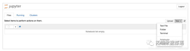
First, import the required libraries:
import warnings
import itertools
import pandas as pd
import numpy as np
import statsmodels.api as sm
import matplotlib.pyplot as plt
plt.style.use('fivethirtyeight')
We will use the CO2 dataset, which collects CO2 samples from March 1958 to December 2001. We can import this data as follows:
y = data.dataLet’s preprocess the data a bit. Weekly data can be cumbersome due to the short time span, so let’s use monthly averages. We can also use the fillna() function to ensure there are no missing values in the time series.
# The 'MS' string groups the data by the start of each month
y = y['co2'].resample('MS').mean()

# Fill missing values
y = y.fillna(y.bfill())
Output
co2
1958-03-01 316.100000
1958-04-01 317.200000
1958-05-01 317.433333
...
2001-11-01 369.375000
2001-12-01 371.020000Let’s visualize the data to explore this time series:
plt.show()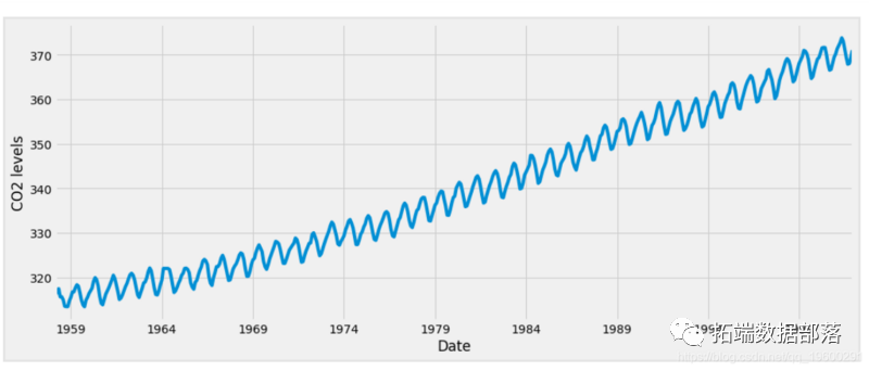
When we plot the data, we can see that the time series exhibits a clear seasonal pattern, and the overall trend is upward.
Click the title to check previous content

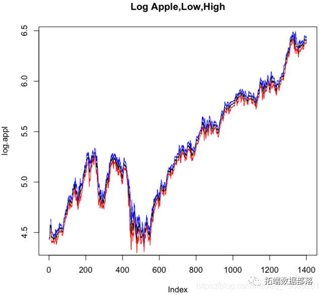
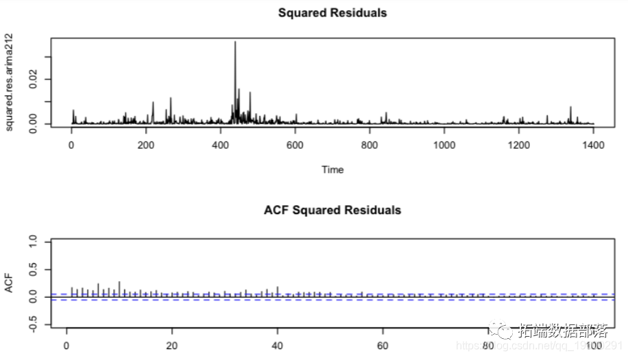
Time series analysis models in R: ARIMA-ARCH/GARCH model analysis of stock prices

Swipe left to see more

01
02
03
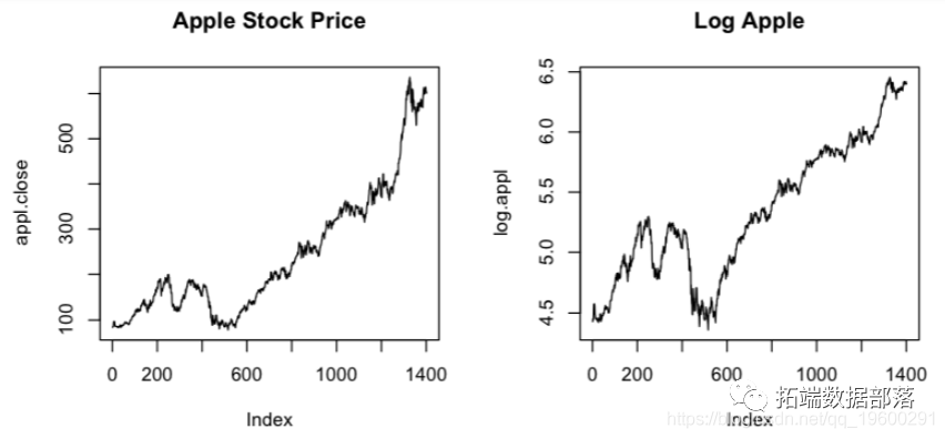
04
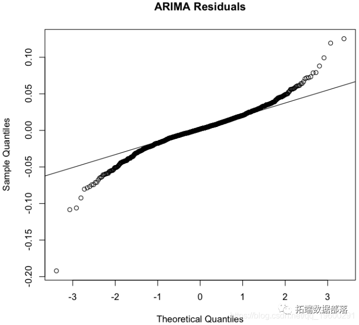
Now, we continue with ARIMA for time series forecasting.
Step 3 – ARIMA Time Series Model
The most common method used in time series forecasting is known as the ARIMA model. ARIMA is a model that can fit time series data to better understand or predict future points in the series.
There are three different integers (<span>p</span>, <span>d</span>, <span>q</span>) used to parameterize the ARIMA model. Thus, the ARIMA model is represented as <span>ARIMA(p, d, q)</span>. These three parameters together describe the seasonality, trend, and noise in the dataset:
-
<span>p</span>is the _autoregressive_ part of the model. It allows us to incorporate the influence of past values into the model. Intuitively, this is similar to stating that if the weather has been warm for the past three days, it is likely to be warm tomorrow. -
<span>d</span>is the differencing part of the model. It contains the amount of differencing to be applied to the time series (i.e., the number of past time points to subtract from the current value). Intuitively, this is similar to stating that if the temperature has varied little over the past three days, tomorrow’s temperature is likely to be the same. -
<span>q</span>is the _moving average_ part of the model. This allows us to set the model’s error as a linear combination of the error values observed at previous time points.
When dealing with seasonal effects, we use _seasonal_ ARIMA (represented as) <span>ARIMA(p,d,q)(P,D,Q)s</span>. Here, <span>(p, d, q)</span> are the non-seasonal parameters, while <span>(P, D, Q)</span> follow the same definitions but apply to the seasonal component of the time series. The term <span>s</span> is the periodicity of the time series (<span>4</span> quarters, <span>12</span> months per year).
Related Videos
In the next section, we will describe the process of automatically identifying the best parameters for the seasonal ARIMA time series model.
Step 4 – Parameter Selection for ARIMA Time Series Model
When we want to fit time series data using a seasonal ARIMA model, our primary goal is to find the values of <span>ARIMA(p,d,q)(P,D,Q)s</span><code><span> that optimize the target metric. There are many criteria and best practices to achieve this, but correctly parameterizing the ARIMA model can be a tedious manual process that requires domain expertise and time. Other statistical programming languages (e.g., </span><code><span>R</span>) provide automated methods to solve this problem, but these methods have not yet been ported to Python. In this section, we will address this issue by programmatically selecting the best parameter values for the <span>ARIMA(p,d,q)(P,D,Q)s</span><span> time series model.</span>
We will use a “grid search” to iteratively explore different combinations of parameters. For each parameter combination, we will fit a new seasonal ARIMA model using the <span>SARIMAX()</span> function from the module. Once the entire parameter space is explored, our best parameter set will be the one that produces the best performance. Let’s first generate the various parameter combinations we want to evaluate:
# Define p, d, and q parameters to take any value between 0 and 2
p = d = q = range(0, 2)

# Generate all different combinations of p, d, and q triples
pdq = list(itertools.product(p, d, q))

# Generate all different seasonal p, d, and q combinations
seasonal_pdq = [(x[0], x[1], x[2], 12) for x in list(itertools.product(p, d, q))]
Output
Examples of parameter combinations for Seasonal ARIMA...
SARIMAX: (0, 0, 1) x (0, 0, 1, 12)
SARIMAX: (0, 0, 1) x (0, 1, 0, 12)
SARIMAX: (0, 1, 0) x (0, 1, 1, 12)
SARIMAX: (0, 1, 0) x (1, 0, 0, 12)Now, we can automate the process of training and evaluating ARIMA models on different combinations using the parameter triples defined above. In statistics and machine learning, this process is known as grid search (or hyperparameter optimization) for model selection.
When evaluating and comparing statistical models with different parameters, each model can be ranked based on how well it fits the data or its ability to accurately predict future data points. We will use the <span>AIC</span> (Akaike Information Criterion) value, which can be conveniently returned by the fitted ARIMA model using <span>statsmodels</span>. The <span>AIC</span> measures the degree to which the model fits the data while considering the overall complexity of the model. A model with fewer features achieving the same goodness of fit will have a lower AIC score compared to a model with many features. Therefore, we look for the model that produces the lowest <span>AIC</span>.
The following code block iterates through the parameter combinations and fits the corresponding Seasonal ARIMA model using the <span>SARIMAX</span> function from <span>statsmodels</span>. After fitting each <span>SARIMAX()</span> model, the code will output their respective <span>AIC</span> scores.
warnings.filterwarnings("ignore") # Specify to ignore warning messages

        try:
            mod = sm.tsa.statespace.SARIMAX(y,
order=param,
seasonal_order=param_seasonal,
enforce_stationarity=False,
enforce_invertibility=False)
The output of the above code produces the following results:
Output
SARIMAX(0, 0, 0)x(0, 0, 1, 12) - AIC:6787.3436240402125
SARIMAX(0, 0, 0)x(0, 1, 1, 12) - AIC:1596.711172764114
SARIMAX(0, 0, 0)x(1, 0, 0, 12) - AIC:1058.9388921320026
SARIMAX(0, 0, 0)x(1, 0, 1, 12) - AIC:1056.2878315690562
SARIMAX(0, 0, 0)x(1, 1, 0, 12) - AIC:1361.6578978064144
SARIMAX(0, 0, 0)x(1, 1, 1, 12) - AIC:1044.7647912940095
...
...
...
SARIMAX(1, 1, 1)x(1, 0, 0, 12) - AIC:576.8647112294245
SARIMAX(1, 1, 1)x(1, 0, 1, 12) - AIC:327.9049123596742
SARIMAX(1, 1, 1)x(1, 1, 0, 12) - AIC:444.12436865161305
SARIMAX(1, 1, 1)x(1, 1, 1, 12) - AIC:277.7801413828764
The output of the code indicates that the <span>SARIMAX(1, 1, 1)x(1, 1, 1, 12)</span> has the lowest <span>AIC</span> value of 277.78. Therefore, among all the models we considered, we should regard it as the best choice.
Step 5 – Fit the ARIMA Time Series Model
Using grid search, we have identified a set of parameters that produce the best fitting model for our time series data. We can proceed to analyze this model in more depth.
We will start by inserting the best parameter values into a new <span>SARIMAX</span> model:
results = mod.fit()Output
==============================================================================
coef std err z P>|z| [0.025 0.975]
------------------------------------------------------------------------------
ar.L1 0.3182 0.092 3.443 0.001 0.137 0.499
ma.L1 -0.6255 0.077 -8.165 0.000 -0.776 -0.475
ar.S.L12 0.0010 0.001 1.732 0.083 -0.000 0.002
ma.S.L12 -0.8769 0.026 -33.811 0.000 -0.928 -0.826
sigma2 0.0972 0.004 22.634 0.000 0.089 0.106
==============================================================================<span>summary</span> output produces a wealth of information returned by the <span>SARIMAX</span>, but we will focus on the coefficients. The <span>coef</span> column shows the weight (i.e., importance) of each function and how each function affects the time series. The <span>P>|z|</span> column informs us of the significance of each feature’s weight. Here, the p-values for each weight are less than or close to <span>0.05</span>, so it is reasonable to keep all weights in our model.
When fitting a seasonal ARIMA model, it is important to run model diagnostics to ensure that the assumptions made by the model are not violated.
plt.show()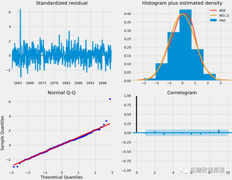
We are primarily concerned with ensuring that the model’s residuals are uncorrelated and normally distributed with a mean of zero. If the seasonal ARIMA model does not meet these properties, it indicates that it can be further improved.
In this case, our model diagnostics suggest that the residuals are normally distributed based on the following:
-
In the upper right plot, we see the red line of the
<span>KDE</span>close to the<span>N(0,1)</span>red line, (where<span>N(0,1)</span>is the normal distribution with mean<span>0</span>and standard deviation of 1). This indicates that the residuals are well approximated by a normal distribution. -
The qq-plot in the lower left shows that the residuals (blue points) follow a standard normal distribution. This also indicates that the residuals are normally distributed.
-
The residuals over time (upper left plot) do not show any obvious seasonal variation but rather white noise. The autocorrelation plot in the lower right confirms this, indicating that the time series residuals have low correlation.
These observations lead us to conclude that our model produces a satisfactory fit that can help us understand the time series data and predict future values.
Although we have a satisfactory fit, certain parameters of the seasonal ARIMA model can be changed to improve the model fit. Therefore, if we expand the grid search range, we may find a better model.
Step 6 – Validate Predictions
We have obtained a model for the time series, and now we can use it to generate predictions. We will first compare the predicted values with the actual values of the time series, which will help us understand the accuracy of the predictions.
pred_ci = pred.conf_int()The above code indicates that predictions start from January 1998.
We can plot the actual values and predicted values of the CO2 time series to evaluate our performance.
 ax.fill_between(pred_ci.index,
                pred_ci.iloc[:, 0],
                pred_ci.iloc[:, 1], color='k', alpha=.2)

plt.show()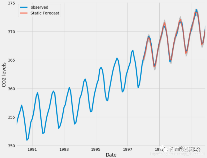
Overall, our predictions align very closely with the actual values, showing an overall upward trend.
It is also useful to quantify our prediction accuracy. We will use MSE (Mean Squared Error) to summarize the average error of our predictions. For each predicted value, we calculate the difference from the actual value and square the result. Squaring the results ensures that positive and negative differences do not cancel each other out when calculating the overall mean.
y_truth = y['1998-01-01':]

# Calculate Mean Squared Error
mse = ((y_forecasted - y_truth) ** 2).mean()
Output
Our prediction mean squared error is 0.07The MSE value obtained from our one-step-ahead prediction is <span>0.07</span>, which is very low as it is close to 0. If the MSE were 0, it would indicate that the estimates predict the observed values with ideal accuracy, which is the ideal case, but this is usually not possible.
However, using dynamic predictions can better represent our true predictive ability. In this case, we only use information from the time series up to a certain point, and thereafter, we will use values from previous forecast time points to generate predictions.
In the code block below, we specify to start calculating dynamic predictions and confidence intervals from January 1998.
By plotting the observed values and predicted values of the time series, we can see that even with dynamic predictions, the overall predictions are accurate. All predicted values (red line) are very close to the actual values (blue line) and fall within our predicted confidence intervals.
We again quantify the prediction performance by calculating the MSE:
# Extract predicted values and actual values from the time series
y_forecasted = pred_dynamic.predicted_mean
y_truth = y['1998-01-01':]

# Calculate Mean Squared Error
mse = ((y_forecasted - y_truth) ** 2).mean()
print('The Mean Squared Error of our forecasts is {}'.format(round(mse, 2)))
Output
Our prediction mean squared error is 1.01The MSE obtained from the predictions generated by dynamic forecasting is 1.01. This is slightly higher than the previous one, which is to be expected since we rely on less historical data from the time series.
Both one-step-ahead and dynamic predictions confirm that this time series model is effective. However, the interest in time series forecasting lies in the ability to predict future values ahead of time.
Step 7 – Generate and Visualize Predictions
Finally, we describe how to use the seasonal ARIMA time series model to predict future data.
# Get predictions for the next 500 steps
pred_uc = results.get_forecast(steps=500)

# Get the confidence intervals for the predictions
pred_ci = pred_uc.conf_int()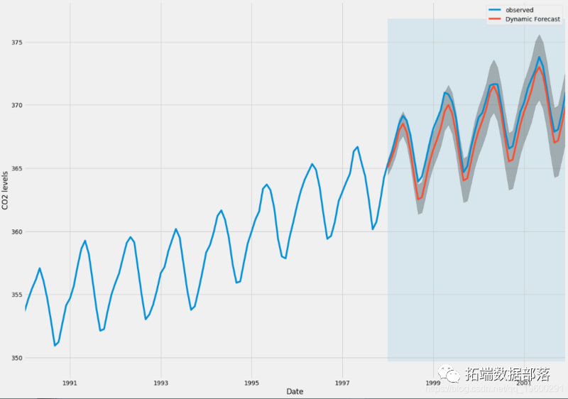
We can use the output of this code to plot the time series and predict its future values.
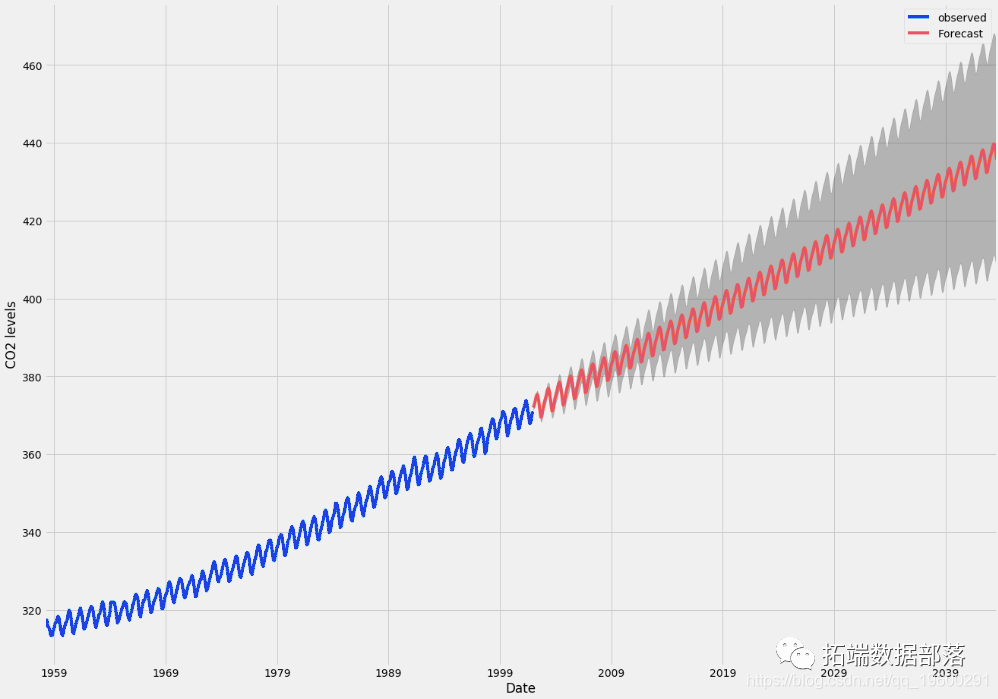
Now, the predictions we generate and the associated confidence intervals can be used to gain further insights into the time series and predict expected outcomes. Our predictions indicate that the time series is expected to continue growing steadily.
As we make further predictions into the future, the confidence intervals will widen.
Conclusion
In this tutorial, we described how to implement a seasonal ARIMA model in Python. We demonstrated how to perform model diagnostics and how to generate predictions for the CO2 time series.
You can try the following additional operations:
-
Change the start date of the dynamic predictions to see how this affects the overall quality of the predictions.
-
Try more parameter combinations to see if you can improve the model’s goodness of fit.
-
Select other metrics to choose the best model. For example, we used
<span>AIC</span>to find the best model.

The data and code analyzed in this article are shared in the member group. Scan the QR code below to join the group!


This article is excerpted from “ARIMA Model Prediction of CO2 Concentration Time Series – Python Implementation“, click “Read the original text” to get the complete materials.


Click the title to check previous content
R language ARIMA-GARCH volatility model predicts daily returns of Apple Inc. stock market time seriesTime series analysis models in R: ARIMA-ARCH/GARCH model analysis of stock pricesMultivariate Copula GARCH model time series prediction in RCopula in Python: Estimation and visualization of Frank, Clayton, and Gumbel copula modelsFitting time series with copula GARCH models in R and simulation analysisUsing Copula simulation in MATLAB to optimize market risk data VaR analysisMultivariate Copula GARCH model time series prediction in RModeling stock market correlation with Copula functions in R: Simulating Random WalkCase study report on Copula algorithm modeling dependency in RARMA-GARCH-COPULA model and financial time series case in RBayesian hierarchical mixture model diagnostic accuracy study based on copula in RCOPULAS and financial time series case in RUsing Copula simulation in MATLAB to optimize market risk data VaR analysisUsing Copula simulation in MATLAB to optimize market riskMultivariate Copula GARCH model time series prediction in RBayesian nonparametric MCMC estimation of Copula in RCOPULAS and financial time series in RMultiplicative GARCH model for high-frequency trading data volatility prediction in RGARCH-DCC model and DCC (MVT) modeling estimation in RUsing GARCH, EGARCH, GJR-GARCH models and Monte Carlo simulation for stock price prediction in PythonTime series GARCH model analysis of stock market volatility in RARMA-EGARCH model, ensemble forecasting algorithm for predicting actual volatility of SPX in RImplementing MCMC for Markov switching ARMA-GARCH model estimation in MATLABUsing GARCH, EGARCH, GJR-GARCH models and Monte Carlo simulation for stock price prediction in PythonUsing R to implement ARIMA + GARCH trading strategy for S&P 500 stock indexModeling financial time series data with multivariate ARMA, GARCH, EWMA, ETS, and stochastic volatility SV models in RExploratory analysis of stock market index: ARMA-GARCH model and log return data in RMultivariate Copula GARCH model time series prediction in RMeasuring market risk with multivariate AR-GARCH model in RTime series analysis models in R: ARIMA-ARCH/GARCH model analysis of stock pricesAnalyzing stock prices with Garch models and regression models in RComparison of VaR using GARCH (1,1), MA, and historical simulation methodEstimating arma garch conditional mean and variance models in MATLABARMA-GARCH-COPULA model and financial time series case in R
To obtain the full text file, please click the lower left corner “Read the original text“.




To obtain the full text file, please click the lower left corner “Read the original text“.