About Reprint Authorization
This is a work from Big Data Digest. Individuals are welcome to share it in their social circles. Media and organizations must apply for authorization for reprints. Please leave a message in the background with “Organization Name + Article Title + Reprint”. Those who have already applied for authorization do not need to apply again, as long as they reprint according to the agreement. However, a QR code for Big Data Digest must be placed at the end of the article.
Compiled by:She YanyaoProgram Comments: Xi XiongfengProofread by: Ding Xue
Original link:https://github.com/python-visualization/folium/blob/master/README.rst
Folium is an open-source library built on the data wrangling capabilities of the Python ecosystem and the mapping capabilities of the Leaflet.js library. It allows you to process data with Python and then visualize it on a Leaflet map.
Concept
Folium makes it easy to visualize data processed by Python on interactive Leaflet maps. It can not only display data distribution maps but also use Vincent/Vega to add markers on the map.
This open-source library includes many built-in map components from OpenStreetMap, MapQuest Open, MapQuest Open Aerial, Mapbox, and Stamen, and supports customizing map components using Mapbox or Cloudmade API keys. Folium supports overlaying both GeoJSON and TopoJSON file formats, and can connect data to these two file format layers, finally allowing the creation of distribution maps using the color-brewer color scheme.
Installation
Install the folium package
Start creating maps
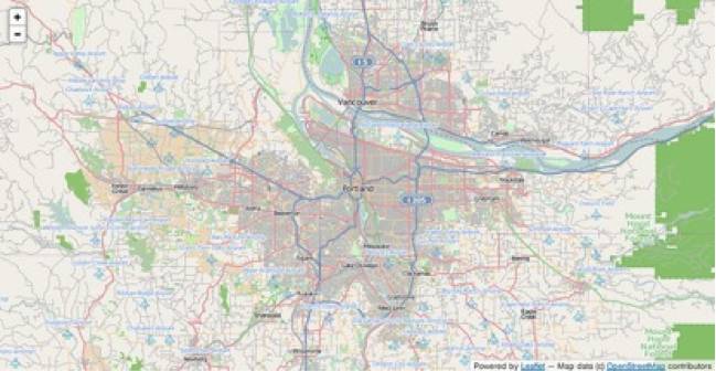
Create a base map by passing the starting coordinates to the Folium map:
import folium
map_osm = folium.Map(location=[45.5236, -122.6750]) #Input coordinates
map_osm.create_map(path=’osm.html’)
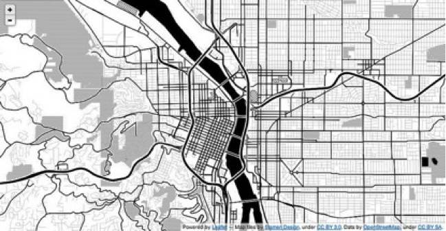
Folium defaults to using the OpenStreetMap component, but Stamen Terrain, Stamen Toner, Mapbox Bright and Mapbox Control spatial components are built-in:
#Input location, tiles, zoom level
stamen = folium.Map(location=[45.5236, -122.6750], tiles=’Stamen Toner’, zoom_start=13)
stamen.create_map(path=’stamen_toner.html’) #Save image
Folium also supports personalized map components from Cloudmade and Mapbox, simply by passing the API_key:
custom = folium.Map(location=[45.5236, -122.6750], tiles=’Mapbox’,
API_key=’wrobstory.map-12345678′)
Finally, Folium supports passing any personalized map components compatible with Leaflet.js:
tileset = r’http://{s}.tiles.yourtiles.com/{z}/{x}/{y}.png’
map = folium.Map(location=[45.372, -121.6972], zoom_start=12,
tiles=tileset, attr=’My Data Attribution’)
Map Markers
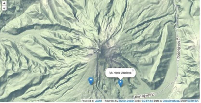
Folium supports drawing various types of markers, starting with a simple Leaflet type location marker with a popup text:
map_1 = folium.Map(location=[45.372, -121.6972], zoom_start=12,
tiles=’Stamen Terrain’)
map_1.simple_marker([45.3288, -121.6625], popup=’Mt. Hood Meadows’) #Text marker
map_1.simple_marker([45.3311, -121.7113], popup=’Timberline Lodge’)
map_1.create_map(path=’mthood.html’)
Folium supports various colors and marker icon types:
map_1 = folium.Map(location=[45.372, -121.6972], zoom_start=12, tiles=’Stamen Terrain’)
map_1.simple_marker([45.3288, -121.6625], popup=’Mt. Hood Meadows’, marker_icon=’cloud’) #Marker icon type is cloud
map_1.simple_marker([45.3311, -121.7113], popup=’Timberline Lodge’, marker_color=’green’) #Marker color is green
map_1.simple_marker([45.3300, -121.6823], popup=’Some Other Location’, marker_color=’red’, marker_icon=’info-sign’)
#Marker color is red, marker icon is “info-sign”)
map_1.create_map(path=’iconTest.html’)
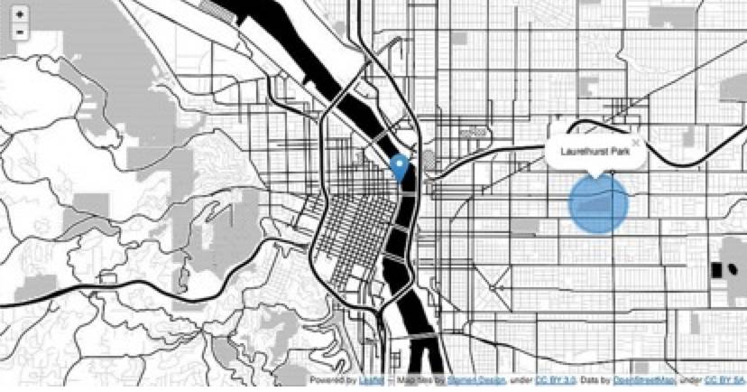
Folium also supports circular markers with personalized sizes and colors:
map_2 = folium.Map(location=[45.5236, -122.6750], tiles=’Stamen Toner’,
zoom_start=13)
map_2.simple_marker(location=[45.5244, -122.6699], popup=’The Waterfront’)
Simple Leaflet Type Marker
map_2.circle_marker(location=[45.5215, -122.6261], radius=500,
popup=’Laurelhurst Park’, line_color=’#3186cc’,
fill_color=’#3186cc’) #Circle marker
map_2.create_map(path=’portland.html’)
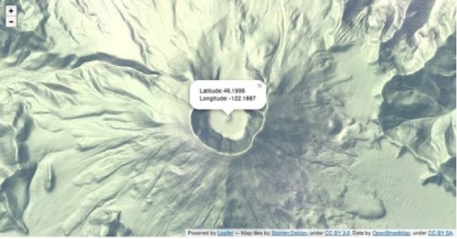
Folium has a convenient feature that allows latitude/longitude to hover over the map:
map_3 = folium.Map(location=[46.1991, -122.1889], tiles=’Stamen Terrain’, zoom_start=13)
map_3.lat_lng_popover()
map_3.create_map(path=’sthelens.html’)
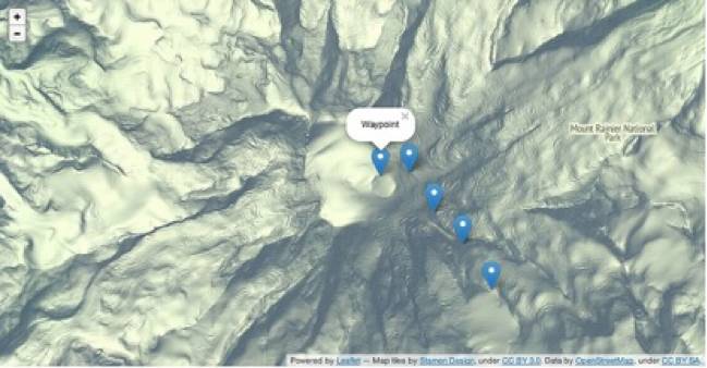
Click-for-marker feature allows dynamic placement of markers:
map_4 = folium.Map(location=[46.8527, -121.7649], tiles=’Stamen Terrain’, zoom_start=13)
map_4.simple_marker(location=[46.8354, -121.7325], popup=’Camp Muir’)
map_4.click_for_marker(popup=’Waypoint’)
map_4.create_map(path=’mtrainier.html’)
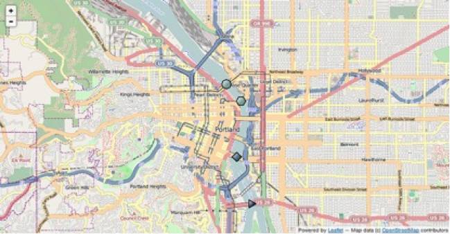
Folium also supports Polygon markers from Leaflet-DVF:
map_5 = folium.Map(location=[45.5236, -122.6750], zoom_start=13)
map_5.polygon_marker(location=[45.5012, -122.6655], popup=’Ross Island Bridge’, fill_color=’#132b5e’, num_sides=3, radius=10) #Triangle marker
map_5.polygon_marker(location=[45.5132, -122.6708], popup=’Hawthorne Bridge’, fill_color=’#45647d’, num_sides=4, radius=10) #Quadrilateral marker
map_5.polygon_marker(location=[45.5275, -122.6692], popup=’Steel Bridge’, fill_color=’#769d96′, num_sides=6, radius=10) #Hexagonal marker
map_5.polygon_marker(location=[45.5318, -122.6745], popup=’Broadway Bridge’, fill_color=’#769d96′, num_sides=8, radius=10) #Octagonal marker
map_5.create_map(path=’bridges.html’)
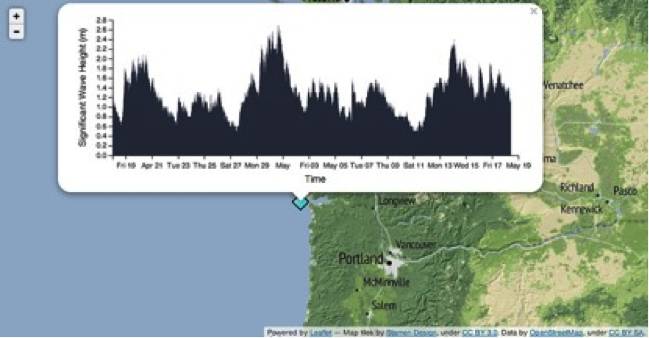
Vincent/Vega Markers
Folium can use vincent to create any type of marker and float it on the map.
buoy_map = folium.Map(location=[46.3014, -123.7390], zoom_start=7,
tiles=’Stamen Terrain’)
buoy_map.polygon_marker(location=[47.3489, -124.708], fill_color=’#43d9de’, radius=12, popup=(vis1, ‘vis1.json’))
buoy_map.polygon_marker(location=[44.639, -124.5339], fill_color=’#43d9de’, radius=12, popup=(vis2, ‘vis2.json’))
buoy_map.polygon_marker(location=[46.216, -124.1280], fill_color=’#43d9de’, radius=12, popup=(vis3, ‘vis3.json’))
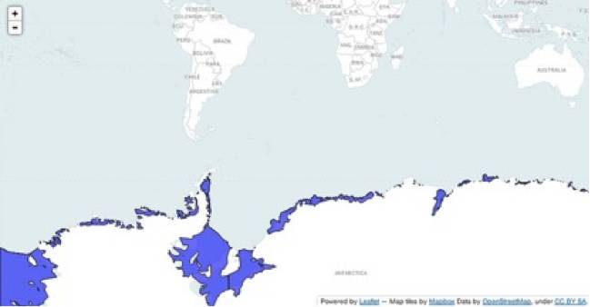
GeoJSON/TopoJSON Layer Overlays
GeoJSON and TopoJSON layers can be imported into the map, and different layers can be visualized on the same map:
geo_path = r’data/antarctic_ice_edge.json’
topo_path = r’data/antarctic_ice_shelf_topo.json’
ice_map = folium.Map(location=[-59.1759, -11.6016], tiles=’Mapbox Bright’, zoom_start=2)
ice_map.geo_json(geo_path=geo_path) #Import geoJson layer
ice_map.geo_json(geo_path=topo_path, topojson=’objects.antarctic_ice_shelf’) #Import TopoJSON layer
ice_map.create_map(path=’ice_map.html’)
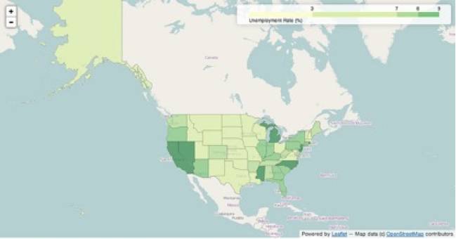
Distribution Maps
Folium allows data conversion between Pandas DataFrames/Series and Geo/TopoJSON types. The Color Brewer color scheme is also built into this library for quick visualization of different combinations:
import folium
import pandas as pd
state_geo = r’data/us-states.json’ #Geographic location file
state_unemployment = r’data/US_Unemployment_Oct2012.csv’ #US unemployment rate file
state_data = pd.read_csv(state_unemployment)
#Let Folium determine the scale
map = folium.Map(location=[48, -102], zoom_start=3)
map.geo_json(geo_path=state_geo, data=state_data,
columns=[‘State’, ‘Unemployment’],
key_on=’feature.id’,
fill_color=’YlGn’, fill_opacity=0.7, line_opacity=0.2,
legend_name=’Unemployment Rate (%)’)
map.create_map(path=’us_states.html’)
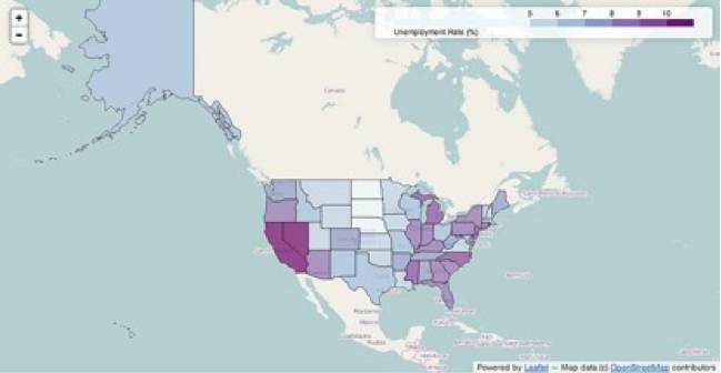
Based on D3 threshold scales, Folium creates legends in the upper right corner, making it easy to import set thresholds:
map.geo_json(geo_path=state_geo, data=state_data,
columns=[‘State’, ‘Unemployment’],
threshold_scale=[5, 6, 7, 8, 9, 10],
key_on=’feature.id’,
fill_color=’BuPu’, fill_opacity=0.7, line_opacity=0.5,
legend_name=’Unemployment Rate (%)’,
reset=True)
map.create_map(path=’us_states.html’)
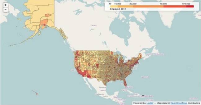
By processing data through Pandas DataFrame, you can quickly visualize different datasets. In the example below, df DataFrame contains 6 columns of different economic data, and we will visualize a portion of the data:
2011 Employment Rate Distribution Map
map_1 = folium.Map(location=[48, -102], zoom_start=3)
map_1.geo_json(geo_path=county_geo, data_out=’data1.json’, data=df,
columns=[‘GEO_ID’, ‘Employed_2011′], key_on=’feature.id’,
fill_color=’YlOrRd’, fill_opacity=0.7, line_opacity=0.3,
topojson=’objects.us_counties_20m’) #2011 Employment Rate Distribution Map
map_1.create_map(path=’map_1.html’)
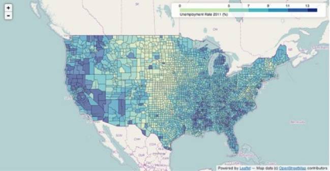
2011 Unemployment Rate Distribution Map
map_2 = folium.Map(location=[40, -99], zoom_start=4)
map_2.geo_json(geo_path=county_geo, data_out=’data2.json’, data=df,
columns=[‘GEO_ID’, ‘Unemployment_rate_2011’],
key_on=’feature.id’,
threshold_scale=[0, 5, 7, 9, 11, 13],
fill_color=’YlGnBu’, line_opacity=0.3,
legend_name=’Unemployment Rate 2011 (%)’,
topojson=’objects.us_counties_20m’) #2011 Unemployment Rate Distribution Map
map_2.create_map(path=’map_2.html’)
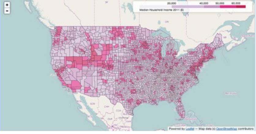
2011 Median Household Income Distribution Map
map_3 = folium.Map(location=[40, -99], zoom_start=4)
map_3.geo_json(geo_path=county_geo, data_out=’data3.json’, data=df,
columns=[‘GEO_ID’, ‘Median_Household_Income_2011’],
key_on=’feature.id’,
fill_color=’PuRd’, line_opacity=0.3,
legend_name=’Median Household Income 2011 ($)’,
topojson=’objects.us_counties_20m’) #2011 Median Household Income Distribution Map
map_3.create_map(path=’map_3.html’)
About the Compiler
Reply “Volunteer” to learn about us and how to join us


Recommended Previous Articles, click the image to read
-
Tested, a step-by-step guide to using Python to grab tickets

-
Step-by-step guide to analyzing WeChat group chat records, identifying troublemakers

-
Step-by-step, 74 lines of code to achieve handwritten digit recognition

[Limited Time Download]
Click the image below to read “7 Major Trends in Big Data Development in 2016”

Before 2016/1/31
For the December 2015 resource file package download, please click the bottom menu of Big Data Digest: Download etc.–December Download
Exciting articles from Big Data Digest:
Reply 【Finance】 to see historical journal articles from the 【Finance and Business】 column
Reply 【Visualization】 to experience the perfect combination of technology and art
Reply 【Security】 for fresh cases about leaks, hackers, and offense-defense
Reply 【Algorithm】 for interesting and informative stories
Reply 【Google】 to see its initiatives in the field of big data
Reply 【Academician】 to see how many academicians discuss big data
Reply 【Privacy】 to see how much privacy remains in the era of big data
Reply 【Medical】 to view 6 articles in the medical field
Reply 【Credit】 for four articles on big data credit topics
Reply 【Big Country】 for the “Big Data National Archives” of the US and 12 other countries
Reply 【Sports】 for applications of big data in tennis, NBA, etc.
Reply 【Volunteer】 to learn how to join Big Data Digest
Long press the fingerprint to follow “Big Data Digest”

Focusing on big data, sharing daily