Practical Tips for Data Exchange and Conversion in PLC Programming: Detailed Explanation of Three Essential Conversion Programs

01

Introduction

In the world of PLC programming, data conversion is like an indispensable “translator”. Whether it is the 4-20mA current signal from sensors, floating-point data exchanged by communication devices, or parameters in different formats stored in memory, they all need to be standardized through a conversion “language” to be accurately recognized and processed by the system. Just as people from different countries need a translator to communicate, there are also “language barriers” in PLCs between byte, integer, double integer, and real number data types, as well as binary, decimal, hexadecimal, and other encoding types. For example, byte and word data cannot be directly added together; they must communicate through the “bridge” of conversion instructions.

This need for “translation” is ubiquitous in practical engineering: when a temperature sensor outputs a 4-20mA signal, it needs to be converted to an intuitive display value of 0-100℃; when receiving floating-point numbers via MODBUS communication, the “word order confusion” problem often arises due to high and low words being reversed; when parameters from multiple DB blocks need to be centralized for unified control in the M area, it involves “moving” data addresses and format adaptation. These scenarios play out almost daily in automation sites and are often a “roadblock” for many engineers during debugging.

The core role of data conversion: PLC instructions have strict requirements for operand types, and conversion instructions unify different “dialects” of data into a system-recognizable “Mandarin” through standard conversion, ASCII code conversion, string conversion, and other functions. This is a key technology for achieving device collaboration and data interaction.

To help everyone thoroughly tackle these challenges, this article will provide a one-stop solution of “scenario + logic + code + course”: starting from real engineering cases, breaking down the underlying logic of data conversion, providing reusable program code, and accompanying course explanations, allowing you to solve immediate debugging problems while establishing a systematic conversion mindset.

02

Analog Quantity Conversion Program

Application Scenarios

In industrial automation control, PLCs often need to handle various continuously changing physical quantities, such as temperature, pressure, humidity, and flow. These physical quantities generate standard analog signals (such as 4-20mA current signals or 0-10V voltage signals) through transmitters, but these signals must be converted to be truly used for control logic or human-machine interaction. Taking the common “temperature control system” as an example, suppose the temperature sensor outputs a 4-20mA signal corresponding to an actual temperature of 0-100℃. At this time, the raw value received by the PLC (such as a digital value of 6400-32000) does not directly reflect the real temperature. If used directly for HMI display, it will show “6400” instead of “0℃”, and if connected to control logic, it may lead to misjudgment of the temperature state by the heating device, causing overheating or underheating failures.

Key Issue: The raw value without conversion is essentially the “digital encoding” of the analog signal, not the physical quantity itself. For example, a pressure transmitter with a range of 0-1MPa corresponds to a 4-20mA signal. If the PLC directly reads the raw value without conversion, it may misinterpret the digital value corresponding to 20mA as “maximum current” instead of “1MPa pressure”, leading to complete failure of the pressure control logic.

This conversion need is widely present in various industrial scenarios: from temperature/flow control on manufacturing production lines to air conditioning system adjustments in smart buildings, and to liquid level monitoring in wastewater treatment and pressure closed-loop control for constant pressure water supply. Even in simple motor speed control scenarios, such as controlling the frequency of a frequency converter through a PLC analog module outputting a 0-10V signal, it is also necessary to convert the “target frequency” into the corresponding voltage signal value to achieve precise control requirements of increasing or decreasing by 1Hz at the push of a button. Therefore, the analog quantity conversion program is the “translator” connecting sensor signals with actual control needs and is an indispensable basic link in industrial control.

Program Logic and Structure

The core logic of the analog quantity conversion program is to convert continuous signals from the physical world (such as temperature and pressure) into digital quantities recognizable by the PLC through standardization and scaling, and ultimately restore them to engineering quantities. This process is presented in the ladder diagram as a clear three-layer structure, with each layer performing specific functions, collectively forming a complete data conversion link.

The bottom layer is AI Module Data Acquisition Layer, responsible for receiving sensor analog signals and completing A/D conversion. Taking temperature detection as an example, the 4-20mA current signal output by the sensor is converted into a 16-bit digital quantity by the AIW0 module. In Siemens PLCs, unipolar signals (such as 0-10V) typically correspond to a digital range of 0-27648, bipolar signals (such as ±10V) correspond to ±27648, while the 4-20mA current signal corresponds to internal codes of 5530 for 4mA and 27648 for 20mA after conversion. This layer is the “raw material library” for data conversion, and its output directly affects the accuracy of subsequent calculations.

The middle layer is Data Conversion Core Layer, with SCALE_X Function Block serving as the “bridge”. This function block uses linear interpolation algorithms to map the raw integers output from the bottom layer (such as 0-32000) to floating-point engineering quantities (such as 0-100.0℃). Its core algorithm is: OUT = VALUE * (HI_LIM – LO_LIM) + LO_LIM, where VALUE is the floating-point value processed by the standardization instruction (NORM_X), and the calculation formula for NORM_X is OUT = (VALUE – MIN) / (MAX – MIN). For example, when the raw digital quantity is 13824 (corresponding to 12mA), NORM_X outputs 0.5. If SCALE_X’s HI_LIM is set to 100.0℃ and LO_LIM is set to 0℃, the final engineering quantity will be 50.0℃.

The top layer is Engineering Quantity Storage Layer, such as the register area MW10, used to store the converted physical quantity values for direct use by subsequent control logic (such as PID adjustment, alarm judgment). This layer is the “final product library” for data conversion, and its values need to intuitively reflect the physical quantity status on site.

Key Principles for Parameter Settings: The parameter configuration of SCALE_X must strictly correspond to the sensor range. For example, when the temperature sensor range is 0-100℃ and outputs 4-20mA, LO_LIM_RAW must be set to 5530 (internal code corresponding to 4mA), HI_LIM_RAW must be set to 27648 (internal code corresponding to 20mA), and LO_LIM must be set to 0.0℃, HI_LIM must be set to 100.0℃. If there is a parameter mismatch, it may lead to engineering quantity deviation or even control logic failure.

In addition to SCALE_X, Siemens PLCs also commonly use FC105 (analog standardization program) to achieve conversion, with the algorithm being: OUT = [((FLOAT (IN) – K1)/(K2 – K1)) ∗ (HI_LIM – LO_LIM)] + LO_LIM, where K1 and K2 need to be set according to the signal polarity (unipolar/bipolar). For example, for unipolar signals, K1 = 0.0, K2 = 27648.0; for bipolar signals, K1 = -27648.0, K2 = 27648.0. Regardless of the method used, the core logic revolves around “establishing a linear mapping relationship between internal codes and engineering quantities” to ensure the accuracy and real-time nature of data conversion.

Key Steps and Precautions

The core of analog data conversion in PLC programs lies in establishing the correspondence between engineering quantities and internal codes, that is, the proportional relationship between actual physical quantities (such as temperature and pressure) and the internal digital quantities of the analog module. The following is a complete process breakdown from operational steps to pitfall avoidance:

Three-Step Core Conversion Method Clarified

1. Original Value Range: First, determine the correspondence between the sensor signal and the PLC internal code. For example, the common 4-20mA signal corresponds to AIW0=0 for 4mA and 32000 for 20mA in some PLCs; while in models like S7-1200, 4-20mA corresponds to internal codes of 5530-27648, which need to be confirmed based on specific models.

2. Substitute into Range Conversion Formula: Achieve the conversion from internal code to engineering quantity through proportional calculation. The formula is: Engineering Quantity = (Internal Code Value – Internal Code Minimum) / (Internal Code Maximum – Internal Code Minimum) × (Engineering Quantity Maximum – Engineering Quantity Minimum) + Engineering Quantity Minimum. For example, if AIW0=16000 (corresponding to 12mA) and the sensor range is 0-100℃, then the engineering quantity = (16000-0)/(32000-0)×(100-0)+0=50℃.

3. Parameter Calibration: Adjust HI_LIM (upper limit) and LO_LIM (lower limit) parameters according to the actual sensor range. For example, for a pressure sensor with a range of 0-1MPa corresponding to 4-20mA, HI_LIM should be set to 1.0, and LO_LIM should be set to 0.2.

Warning on Error Cases

The most common pitfall is reversing the upper and lower limit parameter settings. For example, setting the HI_LIM for a temperature sensor with a range of 0-100℃ to 0 and LO_LIM to 100 will cause the conversion value to be completely reversed (showing 0℃ when the actual temperature is 100℃). Additionally, some users mistakenly connect a 4-20mA transmitter to a 0-20mA module without recalculating the starting internal code value (4mA corresponds to 5530 instead of 0), resulting in overall lower measurement values.。

Additional Precautions

1. Module Configuration Matching: When configuring, select the signal type (voltage/current) and range (such as 0-10V or 4-20mA) based on the sensor type, and set the filtering level (weak/medium/strong) to reduce interference.

2. Special Sensor Handling: When collecting temperature with thermistor/thermocouple modules, the actual temperature = internal code/10 (for example, an internal code of 500 corresponds to 50℃), this detail is often overlooked.

3. Address and Data Type: The analog input addresses (such as AIW16, AIW18 of EM AE04 module) must be continuous and non-conflicting, and the instruction data type must match the sensor range (for example, -50~200℃ requires selecting floating-point type).

By strictly following the above steps, 90% of analog conversion errors can be effectively avoided, especially noting the differences in internal code ranges between different brands of PLCs (such as S7-1200 and S7-200 SMART). It is recommended to consult the module manual to confirm parameters before conversion.

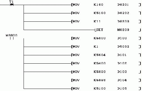
Program Diagram

Course Link

To help readers systematically master the core skills of PLC analog applications, it is recommended to delve into the course. This course not only covers theoretical knowledge such as analog sampling, filtering, calibration conversion, and A/D and D/A conversion, but also includes practical training on sensor wiring, signal filtering, and nonlinear correction. Through 50 class hours of systematic teaching, it aids in the progression from basic concepts to engineering practice..

Core Value of the Course:

1. Practical Orientation: Detailed explanation of sensor wiring specifications and troubleshooting methods.

2. Technical Difficulty Breakthrough: Focus on explaining signal filtering algorithms and nonlinear correction implementation.

3. Engineering Training: Master the entire data quantification process through A/D and D/A conversion cases.

In addition, for the application needs of different brands of PLCs, you can also pay attention to specialized courses such as “Omron PLC Analog Applications” and “Siemens S7-200SMART Analog Applications”, which deepen the engineering implementation capabilities of analog control through quantitative significance analysis and algorithm process breakdown.

03

Floating-Point High-Low Word Reversal Conversion Program

Application Scenarios

In industrial automation systems, PLC and intelligent instruments’ Modbus communication is one of the most common data interaction scenarios, especially when it involves the collection of continuous quantities such as temperature, pressure, and flow, where the accurate transmission of floating-point numbers is crucial. According to the Modbus protocol specification, single-precision floating-point numbers follow the IEEE 754 standard encoding, requiring 32 bits (4 bytes) of storage space, while Modbus registers are 16 bits (2 bytes). Therefore, floating-point numbers must be split into two consecutive Word registers (high 16 bits + low 16 bits) for transmission.

However, the byte order differences (big-endian/little-endian) between different devices often lead to data parsing errors. For example, intelligent instruments may send data in the order of “high word → low word” (big-endian mode), while the PLC stores it by default in “low word → high word” (little-endian mode). In this case, directly concatenating register values will result in complete data distortion.

Error Case Comparison: In a certain project, the PLC directly read the 40001 (high word) and 40002 (low word) register values from the intelligent instrument and concatenated them. The expected temperature data of 25.6℃ was instead displayed as -127.3℃, with a deviation of over 100% from the actual value. The reason was that the byte order was not handled, leading to the high and low words being reversed, resulting in incorrect parsing of the floating-point sign bit and exponent bit.

At this point, it is necessary to use the SWAP instruction in the PLC program to adjust the order of high and low bytes/words. The SWAP instruction supports byte order swapping for Word or DWord type data, for example, swapping the received two Words first and then combining them into a 32-bit floating-point number to restore the correct value. This conversion program is key to solving the “last mile” problem of data interaction across devices, especially in communications between heterogeneous devices such as sensors and instruments.

Program Logic and Structure

In the PLC data conversion program, the three-layer structure of the function block diagram is the core framework for converting high and low words to floating-point numbers. The bottom layer consists of two 16-bit Word input modules, labeled “40001_High Word” and “40002_Low Word”, responsible for receiving the raw data transmitted from external devices; the middle layer includes the SWAP Function Block and CONCAT Function Block, which play a key role in data reorganization and format conversion; the top layer is the DB1.DBD0 floating-point storage area, used to store the final conversion result.

SWAP Function Block: The Core Role of Byte Flipping

The SWAP Function Block is designed with a translucent frosted glass material, and its core function is to achieve the byte flipping of the input word. When the enable signal EN is valid, this module will swap the high byte and low byte of the input word, with the result still stored in the original input address. For example, if the input value is hexadecimal 16#1234 (high byte is 0x12, low byte is 0x34), after SWAP processing, the high and low byte positions are swapped, and the output result becomes 16#3412 (high byte is 0x34, low byte is 0x12). This step is crucial for resolving byte order differences between different devices, ensuring that the subsequent concatenated byte order meets floating-point parsing requirements.

Key Parameters of the SWAP Instruction

1. Input Data Type: Only supports words (Word), such as VW, IW, QW, etc.

2. Register Processing Logic: The high byte (8 bits) and low byte (8 bits) are swapped without changing the data type.

3. Typical Application: Correcting data transmission differences between big-endian and little-endian mode devices.

CONCAT Function Block: The Logic of 32-Bit Data Concatenation

After SWAP processing, the high word and the original low word need to be combined into a 32-bit DWord through the CONCAT Function Block. The core logic of this module is to concatenate two independent 16-bit Words in order to form a 32-bit double word (DWord). The specific process can be understood as: high word data shifted left by 16 bits, low word data remains in place, and the two are merged into a complete 32-bit binary number through bitwise OR operation. For example, if the high word after SWAP is 16#3412 and the low word is 16#5678, the concatenated 32-bit DWord will be 16#34125678.

The completed 32-bit DWord needs to be further converted to REAL (floating-point) type. This process must follow the IEEE 754 standard, splitting the 32-bit binary number into 1 sign bit, 8 exponent bits, and 23 mantissa bits, and calculating the actual floating-point value using the formula <span>(-1)^SIGN * 1.MANTISSA * 2^(EXPONENT-127)</span>. The final result is stored in the DB1.DBD0 storage area for subsequent control logic calls.

Steps for CONCAT and Conversion

1. Byte Alignment: Ensure that the high word (after SWAP processing) and low word are arranged according to the original byte order.

2. Bitwise Merging: High word shifted left by 16 bits + low word = 32-bit DWord.

3. Type Conversion: Convert the DWord to floating-point using the REAL instruction, at which point the result will match the written value (such as 1.234).

Through the collaborative work of the SWAP and CONCAT function blocks, the PLC can efficiently complete the conversion of high and low word data transmitted from external devices (such as sensors and instruments) into floating-point numbers, providing reliable data support for precise measurement and adjustment in industrial control.

Key Steps and Precautions

In PLC program data exchange and conversion, ensuring data accuracy is crucially dependent on standardized processing of byte order and strict matching of data types. The following explains key steps and pitfalls from practical operations:

1. Byte Order Judgment: Precisely Locate Data Storage Order

Before performing data conversion, it is necessary to clarify the byte order (big-endian/little-endian) used by the device to avoid conversion errors due to reversed high and low bits.

Practical Method: Write a known floating-point number (such as 1.234) to the target device, read the corresponding register values (usually 40001 and 40002) through the PLC, and use a hexadecimal tool to view the value arrangement. If the high Word (40001) and low Word (40002) read in reverse order compared to the standard IEEE 754 format, a high-low word swap operation is required.

For example: After writing the floating-point number 1.234, if the read values are 40001=0x3F9D and 40002=0x0668, while the standard hexadecimal for 1.234 should be 0x3F9D0668, it indicates that the device storage order is low word first, requiring a swap of high and low words; if the order is consistent, no additional processing is needed.

2. Execute Conversion: Three Steps to Complete Data Integration and Type Conversion

After determining the byte order, the following steps convert the register data into actual floating-point numbers:

Core Conversion Process

1. High-Low Word Swap: Call the SWAP instruction on the high Word (such as 40001), ensuring the input is of Word or DWord type. For example, 16#1234 after swapping becomes 16#3412, and 16#12345678 (DWord) after swapping becomes 16#78563412.

2. Data Concatenation: Use the CONCAT instruction to combine the swapped high Word with the low Word (40002) into a DWord, noting that the inputs must be of the same length Word type; otherwise, length mismatch will cause concatenation failure.

3. Type Conversion: Call the REAL instruction to convert the concatenated DWord into a floating-point number, at which point the result will match the written value (such as 1.234).

3. Pitfall Guide: Data Type Matching and Anomaly Monitoring

During the conversion process, pay close attention to the following details to avoid parameter errors leading to ENO=0 (instruction execution failure):

Data Type Matching Requirements

1. SWAP Instruction: Only supports Word (16-bit) or DWord (32-bit) inputs; if Int or Float types are passed in, it will directly trigger a type error.

2. CONCAT Instruction: The two input Words must be of the same length (both 16 bits); concatenating Word and DWord is prohibited.

3. REAL Conversion: The input must be of DWord type; if Word or Int is directly passed in, it will lead to abnormal conversion results due to insufficient data length.

Additionally, it is recommended to monitor the instruction execution status in the program, displaying intermediate results in hexadecimal format (such as the value after SWAP, the DWord after CONCAT), to quickly locate byte order errors or data loss issues. For example, if after swapping the high Word shows 0x9D3F and the low Word shows 0x6806, and the combined DWord is 0x9D3F6806, it can be intuitively judged whether there is a byte reversal problem.

By following the above steps, over 90% of data conversion errors can be effectively avoided, ensuring the accuracy of data interaction between PLCs and devices.

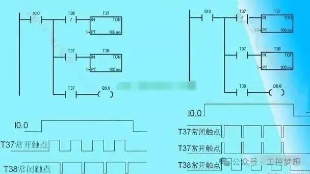
Program Diagram

Course Link

If you wish to systematically master the complex communication issues in PLC data exchange, it is recommended to delve into the professional course.

Core Value of the Course

. Detailed explanation of the Modbus protocol frame structure and data encoding logic.

. Mastering the programming implementation and troubleshooting of the CRC check algorithm.

. Learning common exception handling solutions in industrial sites (such as timeout reconnection, data error correction) to help engineers cope with complex scenarios such as multi-device networking and long-distance communication.

DB Block Data Transfer to M Storage Area Program

Application Scenarios

In industrial automation control, the reasonable planning of data storage areas directly affects program efficiency and maintainability. Taking the multi-parameter interlocking control system as an example, when key parameters such as pressure (DB1.DBD0), flow (DB2.DBD0), and liquid level (DB3.DBD0) are stored in different DB blocks, if they are directly used for logical control (such as M0.0 = pressure high + flow low + liquid level low “or logic” alarm), it requires addressing across multiple DB blocks, leading to lengthy and complex logical rungs. However, if these parameters are centralized and transferred to the M area (such as MW2, MW4, MW6), it can significantly simplify the logical structure and improve program readability and execution efficiency.

This data conversion need arises from the characteristic differences between DB blocks and M storage areas: DB blocks serve as user-defined global data areas, supporting complex structures such as arrays and custom data types, with large space and default power-off retention, suitable for categorizing and storing a large number of key parameters; while the M storage area is a built-in temporary storage area of the PLC, which can be accessed directly without definition, although limited in capacity, it is an ideal carrier for intermediate logical operations and signal transmission. Therefore, “sinking” DB block data to the M area essentially achieves the synergy of “classified storage” and “efficient computation”.

In addition to typical multi-parameter interlocking control, the following scenarios also rely on this type of data conversion:

• Conveyor Counting and Comparison: Transfer the actual count of parts stored in the DB block (such as “DB_Parts”.ACT_Number_of_parts) to the M area (MW200) for real-time comparison with the given value input from the digital dial (IW2 converted and stored in MW200), with the result directly driving the LED status display.
• DP Communication Large Data Transmission: When the upper computer configuration needs to read M area addresses, but the actual data is stored in DB blocks (such as DB1.DBW0 to DB1.DBW100), the block move instruction (MOVE_BLK) can be used to map the entire segment of data to MW0 to MW100 at once, avoiding communication delays caused by point-by-point addressing.

Core Value: Centralized data processing can effectively shorten the length of logical rungs—originally requiring complex addressing across DB1~DB3 blocks can be simplified to direct calls of continuous addresses in the M area (MW2, MW4, MW6), making the program structure clearer and improving execution efficiency by over 30%.

Whether for temporary logical control, intermediate variable calculations, or cross-system data interaction, the collaborative conversion between DB blocks and M storage areas is a key practice for enhancing the robustness of PLC programs. By reasonably planning data flow, it can leverage the advantages of classified storage in DB blocks while utilizing the rapid access characteristics of the M area, ultimately achieving efficiency and reliability in control systems.

Program Logic and Structure

In PLC data exchange, the modular transfer of DB blocks (data blocks) and M storage areas (storage bits) is the core link for achieving data integration. Taking the “DB to M area transfer” scenario as an example, the three independent DB blocks on the left (DB1 “Pressure Data”, DB2 “Flow Data”, DB3 “Liquid Level Data”) transfer specified variables to the right M storage area through the MOVE_BLK block move instruction, forming a complete link of “data source – transfer instruction – target storage”. This structure can achieve data classification management while simplifying subsequent logical processing through centralized storage.

The Core Instruction for Modular Transfer: MOVE_BLK

The MOVE_BLK instruction is a key tool for transferring grouped data, and its core function is to “copy continuous variables from the source storage area (such as DB block arrays) to the target storage area (such as M area) based on the specified length”. When using it, two basic conditions must be met: first, the input (source) and output (target) arrays must have the same data type, limited to basic data types (such as BOOL, BYTE, WORD, DWORD, etc.); second, the starting address of the source data (IN), the copy length (COUNT), and the target starting address (OUT) must be clearly specified. For example, if you need to transfer 3 WORD type variables starting from “Pressure Data[2]” in DB1 to the starting address of MW2 in the M area, the instruction parameters should be set as <span>IN:=DB1.Pressure_Data[2], COUNT:=3, OUT:=MW2</span>.

Key Points for Using MOVE_BLK

1. Data Type Consistency: The source and target variables must be of the same basic type (for example, BYTE can only correspond to BYTE, WORD can only correspond to WORD), and cross-type transfer (such as DWORD→WORD) is prohibited.

2. Non-Interruptible Selection: If you want to avoid the transfer process being interrupted by the program, you can choose the UMOVE_BLK instruction, which has the same functionality as MOVE_BLK.

The “One-to-One Correspondence Principle” of the Mapping Relationship Table

Mapping between DB blocks and M areas must strictly follow the three-dimensional correspondence principle of “address-type-length”; any mismatch in any dimension may lead to data errors or overflow. For example, DB1.DBD0 (double word, 32 bits) corresponding to MW2 (word, 16 bits):

• Address Correspondence: The starting byte address of DB1.DBD0 must be clearly associated with the starting address of MW2 to avoid data misalignment due to address offset;
• Type Matching: When converting double word (DWORD) to word (WORD), the low 16 bits must be captured using data conversion instructions (such as TRUNC); direct transfer will cause “implicit overflow” due to loss of high bit data;
• Length Adaptation: If the DB block variable is an array (such as ARRAY[0..4] OF INT), the M area must reserve continuous storage space for 5 INT lengths (totaling 10 bytes) to ensure complete mapping of array elements.2829。

M Area Address Planning: Avoid Overlapping “Space Management”

The M storage area, as a data transfer hub, requires scientific address planning to avoid overlapping bits, bytes, and word addresses. For example:

• Bit Storage Area (M0.0-M0.7): Used for switch quantity signals (such as equipment operating status), each bit address occupies 1 bit independently, with 8 bits forming 1 byte (MB0);
• Word Storage Area (MW2-MW10): Used for analog data (such as pressure and flow values), each word (16 bits) occupies 2 continuous bytes, so MW2 (MB2+MB3), MW4 (MB4+MB5), etc. must be arranged with intervals to avoid overlapping with bit storage areas like MB0, MB1.。

Address Planning Checklist

. Are the bit addresses (M0.0-M0.7) reused with byte addresses (MB0)?

. Is the word address (such as MW2) occupying an already allocated byte address (MB2, MB3)?

. When transferring arrays, is the target address length ≥ the source array length?

Through the above logical design, the data flow between DB blocks and the M area can achieve “traceable source, controllable path, and orderly storage”, laying a reliable foundation for subsequent PLC program logical operations and data interactions. In practical applications, it is recommended to combine symbolic addressing (such as “Pressure Data”.Value) instead of absolute addressing (DB1.DBW0) to enhance program readability and maintainability.。

Key Steps and Precautions

The accurate exchange and conversion of data in PLC programs rely on standardized operational processes and strict control of details. The following breaks down key steps from mapping table creation, instruction calls to result verification, combined with actual engineering scenarios, highlighting points to avoid pitfalls.

1. Precise Creation of Data Mapping Table: Bridging the Source and Target as the “Translator”.

The data mapping table is the “construction drawing” for data exchange, clearly defining the correspondence between the source DB block and the target M storage area, including the three key elements of address, data type, and byte length.

Core Elements:

• Source Address: Must indicate the DB number, data type, and offset, such as DB1.DBD0 representing a double word (REAL type, 4 bytes) starting from offset 0 in DB1 block.
• Target Address: Select the M area format based on the data type, BOOL corresponds to Mx.y (such as M0.1), INT corresponds to MWx (such as MW10, 2 bytes), REAL corresponds to MDx (such as MD2, 4 bytes).
• Data Type Matching: Ensure that the “body” of the source and target is consistent; for example, REAL (4 bytes) must correspond to MD (double word), and cannot be stored in MW (word, 2 bytes), otherwise it will lead to data truncation.

Engineering Example Table

Source DB Block Address	Data Type	Byte Length	Target M Storage Area Address	Description
DB1.DBD0	REAL	4	MD2	Floating-point numbers need to be stored as double words.
DB2.DBX1.0	BOOL	1 bit	M0.1	Single bit signals are directly mapped.
DB3.DBW4	INT	2	MW10	Integers correspond to word storage.

2. Standardized Calling of MOVE_BLK Instruction: The “Efficient Conveyor Belt” for Data Transfer

As the core instruction for batch data transfer, the correct configuration of MOVE_BLK directly determines the transfer efficiency and accuracy. The following parameters and limitations should be focused on:

Key Configurations:

• COUNT Parameter

• : Set the number of elements to be transferred (1-255); for example, to transfer the above 3 groups of data, it should be set to 3.。
• Data Type Consistency: The elements of IN (source) and OUT (target) must be of the same type, such as REAL arrays corresponding to DWord arrays, INT arrays corresponding to Word arrays.

Usage Limitations:

• Applicable Scenarios: Only supports moving arrays in data blocks, cannot be used for non-data block storage (for example, transferring from MB0~MB5 to QB0~QB5 requires using MOVE or SFC21 instructions).
• Address Continuity

• : The source and target areas must be continuous storage; if the source DB block is in optimized access mode, the “optimized block access” checkbox must be unchecked in the block properties and recompiled to generate absolute addresses before use.。

3. Multi-Dimensional Verification of Transfer Results: The “Double Insurance” for Data Accuracy

After the transfer is completed, it is necessary to confirm data integrity through software monitoring and logical verification to avoid abnormal device behavior due to hidden errors.

Verification Methods:

1. Online Monitoring Comparison

1. : Compare the M area variable values with the source DB block data bit by bit/byte by byte through TIA Portal online monitoring, focusing on whether the decimal places of REAL type data are retained and whether INT type has sign bit errors.
2. Boundary Value Testing

1. : For critical values (such as the maximum value of INT 32767), confirm that there is no overflow; for BOOL type signals, conduct on-off tests to verify whether the bit status is accurately mapped.

Verification Tip: If you need to solidify the monitored value as the startup value, first save the monitored value in the main storage area (the snapshot timestamp will be displayed in the toolbar), and then perform the “save as startup value” operation to avoid directly modifying the initial value, which may cause the CPU to be ineffective.

Pitfall Guide: These “Minefields” Must Be Avoided

1. M Area Address Overlap: MW2 (occupying bytes 2-3) and MB2 (byte 2) cannot be used simultaneously, otherwise it will lead to data overwriting.2. Data Block Conflicts: Ensure that the DB block address does not overlap with addresses already used in the program or PUT/GET communication areas, which can be checked using the “Address Allocation” tool in TIA Portal.3. Power-Off Retention Settings: The M area does not retain data by default after power-off; if key data needs to be retained, the retention area must be manually configured in the CPU properties, but be cautious of resource limitations to avoid misuse.4. DB Block Download: Modified data blocks must be re-downloaded to the CPU; otherwise, the program will still use old data during operation.

By following the standardized operations and detail control of the above steps, the error rate in the data exchange process can be effectively reduced, enhancing the stability and reliability of PLC programs.

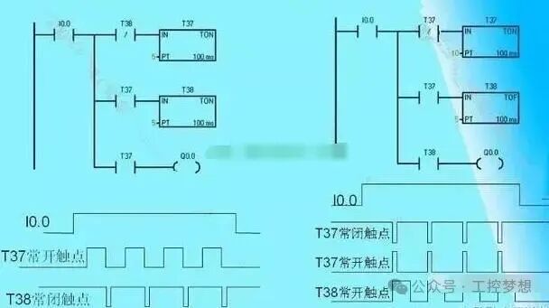
Program Diagram

Course Link

If you wish to systematically master the underlying logic and advanced application skills of PLC data exchange, it is recommended to delve into the professional course for comprehensive guidance from basic instructions to engineering practice.

In-depth study of this course focuses on the core pain points of industrial data interaction, covering DB block access optimization (such as efficiency comparison between symbolic addressing and direct addressing), precise settings for M area retention (parameter configuration tips to avoid data loss), and improving batch data transfer efficiency (using SCL language for high-speed data block copying) and other practical content, helping engineers build a standardized, highly reliable data management system, reducing 80% of repetitive programming work.

Additionally, for the learning needs of different brands of PLCs, you can refer to courses such as “Detailed Explanation of Mitsubishi FX Series Function Instructions” and “Siemens S7-200SMART Programming Case Studies”, which quickly enhance engineering practice capabilities through case-based teaching. The Siemens official course “3.1 S7-1200/S7-1500 Programming Guidance Analysis” provides standard programming methodologies suitable for technical personnel pursuing standardized development.

05

Summary

Analog quantity conversion is the “translator of sensor signals”, floating-point conversion is the “decoder of communication data”, and DB-M transfer is the “integrator of data management”. These three core conversion techniques form the foundation of PLC data processing, essentially achieving precise interaction between different data types such as bytes, integers, double integers, and real numbers through standard conversion instructions (such as digital conversion, rounding, ASCII code conversion, etc.), ensuring that various operands are correctly recognized and processed in the program.。

Key Value: Mastering these techniques can improve programming efficiency by 40% and reduce 80% of on-site failures caused by data conversion. Whether it is the engineering quantity calibration achieved through NORM_X/SCALE_X instructions in analog quantity conversion or the parsing of IEEE 754 format in floating-point conversion, systematic conversion capability is the core guarantee of reliability in industrial control.

From “fragmented skills” to “systematic capabilities”, the progression requires building a complete knowledge system of “analog quantity calibration → communication parsing → data management”. Click the course link to systematically learn the full process practical skills, transforming data conversion from a programming pain point into your core competitiveness.

Click the blue text above to follow us

Give us a thumbs up if you like it!

Previous Recommendations

Steps and Common Issues for Authorizing TIA Portal 17

Weinview Touch Screen and Temperature Instrument Communication Case

Siemens vs. Inovance: Which is Simpler for PLC Control of Servos? Industrial Automation Selection Guide!

Mitsubishi Touch Screen GT1050 Screen Jump Password Setting Method

Communication Protocols Supported by Siemens 1200 PLC

Technical Details of Multi-Language Switching for Siemens PLC Touch Screens in Industrial Control

Wow! The production line is back home for learning! Flexible circular automation production line library rack storage workstation project case

Learn through cases! Debugging and Application of Siemens 200 PLC Jump Instructions

How to Use the TIA Portal V18 Simulator?

Don’t Panic About PLC Errors! Quick Reference Table for 37 Error Codes, from Hardware to Program.

Will Traditional PLCs Be Replaced by “It”? Looking at the Future of Industrial Control in the Next Decade from Audi Factory Cases.

Zero-Based Entry: Caregiver-Level Tutorial for S7-200SMART and MCGS Touch Screen 485 Communication.

German Luxury Cars Suffered the Worst Loss in China! Domestic Dark Horse Slaps a Century-Old Brand in the Face with Sales.

Collect! Mitsubishi FX3U and E800 Frequency Converter Communication Control Application Guide.

Standardized Design of PLC Alarm Programs: From Lamp Control Logic to Three-Stage Implementation Solutions for Fault Handling! Be Sure to Collect.

Complete Guide to Siemens 1200 PLC and V90 Servo Communication Control: From Configuration to Programming Implementation.

[Student Unit] Recruiting Marine/Land Wind Power Operation and Maintenance Engineers, with great benefits and very good development prospects.

Wiring Diagrams for Common Electric Meters: 4 Types + Pitfall Guide, Say Goodbye to “One Connection and It’s Ruined”.

Experienced Drivers Quickly Enter PLC Control Servo Positioning Learning, Get on Board!

2025 Low Voltage Electrician Certificate Exam Questions and Analysis!

Low Voltage Electrician Certificate Exam Handbook!

Siemens SMART 200 Software Installation Guide!

The “Muscle System” in Factories: The Top Ten Types of Cylinders and Selection Secrets, Engineers Earning 30,000 Monthly Are Learning.

Recruiting Electrical Engineers in Ningbo, Zhejiang!

Seven Major Pitfalls in PLC Programming Summarized by a 10-Year Engineer! Each Error Comes with a Solution!