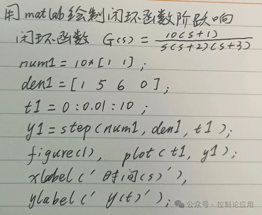
First, input the coefficients of the numerator and denominator polynomials of the closed-loop transfer function, and then use the step function to plot the response curve.
Related posts
- SPI Communication Notes: Basics, Animations, Timing Diagrams, and Summary
- Analysis of the Five Leading Stocks in PLCs, the Core Equipment of Industrial Automation
- Dingo Optimization Algorithm for Single Objective Optimization with MATLAB Code
- Digital Image Input/Output and Display in MATLAB
- Understanding Graph Theory Problems with MATLAB
- Earthquake Response Spectrum Analysis Using MATLAB
- MATLAB | GLASS Global Vegetation Photosynthetically Active Radiation Absorption Ratio FAPAR Data from 1982 to 2018
- MATLAB Signal Processing | Seismic Signal Spectrum Analysis (Complete Code Included)
- MATLAB and COMSOL Coupled Simulation Method (Part 1): Introduction
- Download MATLAB Software Installation Package + Illustrated Installation Guide (Includes All Versions)
- MATLAB T-S Diagram
- Ready-to-Use Academic-Level Plotting 3: Line Graph (MATLAB Implementation, Foolproof Data Replacement)
- Multisim 14.0 Software Installation Package and Detailed Installation Guide
- Parsing XML with Matlab
- Artificial Hummingbird Algorithm for Multi-Objective Optimization with MATLAB Code