New Method PiSSA Significantly Enhances Fine-Tuning Effects

As the parameter count of large models continues to grow, the cost of fine-tuning the entire model has become increasingly unacceptable.

To address this, a research team from Peking University proposed a parameter-efficient fine-tuning method called PiSSA, which surpasses the fine-tuning effects of the widely used LoRA on mainstream datasets.

Paper Link:

Code Link:

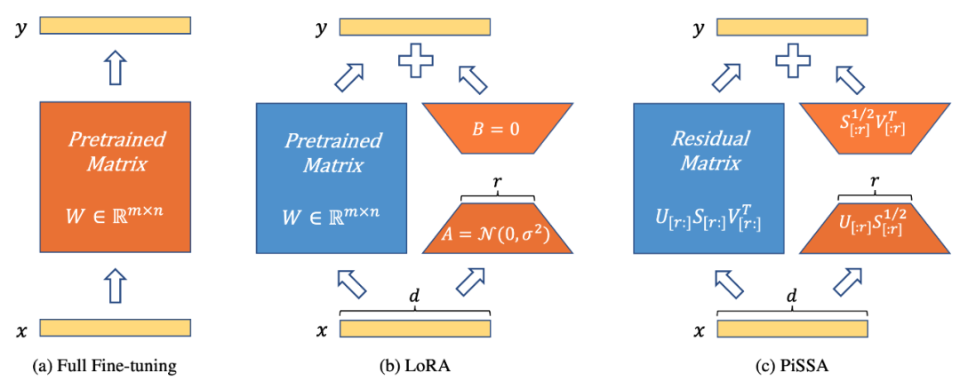
As shown in Figure 1, PiSSA (Figure 1c) is architecturally identical to LoRA [1] (Figure 1b), differing only in the initialization method of the Adapter. LoRA initializes A with Gaussian noise and B with 0. In contrast, PiSSA uses Principal Singular Values and Singular Vectors to initialize A and B.

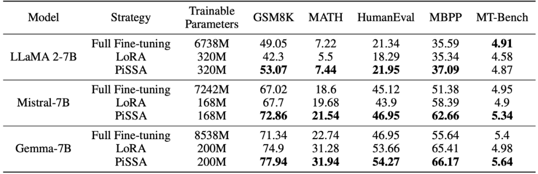
Comparing Fine-Tuning Effects of PiSSA and LoRA on Different Tasks: The research team used llama 2-7B, Mistral-7B, and Gemma-7B as base models to enhance their mathematical, coding, and conversational abilities through fine-tuning. This includes training on MetaMathQA and validating the model’s mathematical capabilities on the GSM8K and MATH datasets; training on CodeFeedBack and validating the model’s coding abilities on HumanEval and MBPP datasets; training on WizardLM-Evol-Instruct and validating the model’s conversational abilities on MT-Bench.

The experimental results in the table below indicate that, using the same scale of trainable parameters, the fine-tuning effect of PiSSA significantly surpasses that of LoRA, even exceeding that of full parameter fine-tuning.

Comparing Fine-Tuning Effects of PiSSA and LoRA Under Different Amounts of Trainable Parameters: The research team conducted ablation experiments on the relationship between the amount of trainable parameters and the effects on mathematical tasks. From Figure 2.1, it can be seen that in the early stages of training, the training loss of PiSSA decreases particularly quickly, while LoRA experiences a phase where the loss does not decrease, and may even slightly increase.

Moreover, the training loss of PiSSA remains lower than that of LoRA throughout, indicating better fitting to the training set; Figures 2.2, 2.3, and 2.4 show that under each setting, the loss of PiSSA is consistently lower than that of LoRA, and the accuracy is consistently higher than that of LoRA, demonstrating that PiSSA can achieve results comparable to full parameter fine-tuning with fewer trainable parameters.

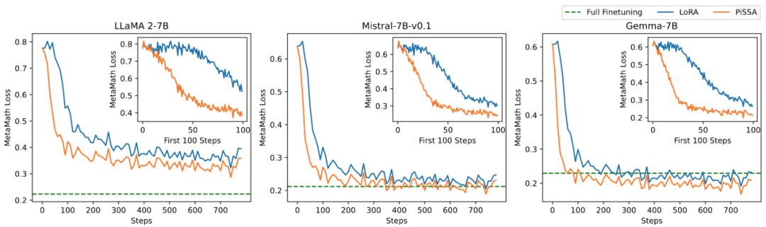
▲ Figure 2.1) When rank is 1, the loss during the training process for PiSSA and LoRA. The upper right corner of each figure shows an enlarged curve for the first 100 iterations. PiSSA is represented by the orange line, LoRA by the blue line, and full parameter fine-tuning by the green line, which shows the final loss for reference. Similar phenomena are observed for ranks [2,4,8,16,32,64,128]; see the appendix of the article for details.

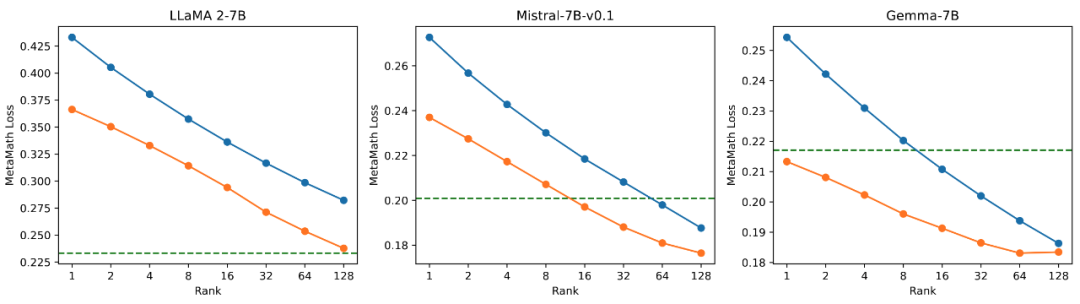
▲ Figure 2.2) The final training loss of PiSSA and LoRA using ranks [1,2,4,8,16,32,64,128].

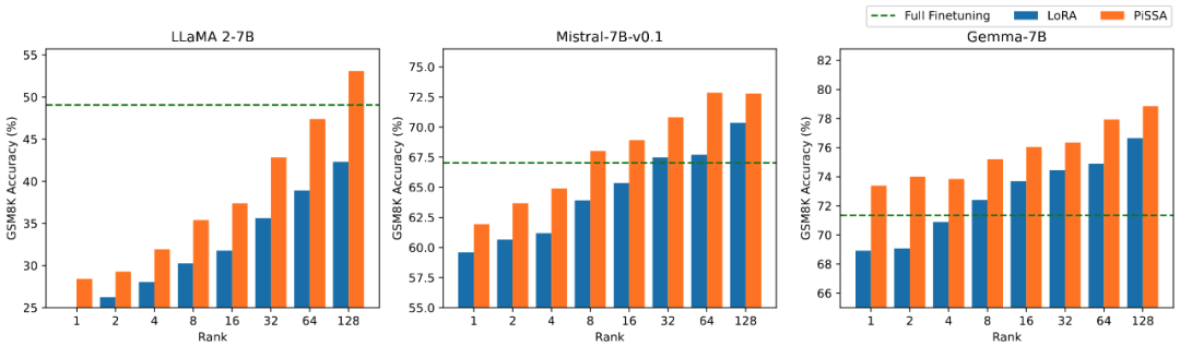
▲ Figure 2.3) The accuracy of models fine-tuned with PiSSA and LoRA on GSM8K using ranks [1,2,4,8,16,32,64,128].

▲ Figure 2.4) The accuracy of models fine-tuned with PiSSA and LoRA on MATH using ranks [1,2,4,8,16,32,64,128].

Inspired by the Intrinsic SAID [2] that “the parameters of pre-trained large models exhibit low-rank characteristics”, PiSSA performs singular value decomposition (SVD) on the parameter matrix of the pre-trained model, where the first r singular values and singular vectors are used to initialize the two matrices of the adapter (adapter) and , while the remaining singular values and singular vectors are used to construct the residual matrix, ensuring that.

Thus, the parameters in the adapter contain the core parameters of the model, while the parameters in the residual matrix are correction parameters. By fine-tuning the smaller number of core adapters A and B, and freezing the larger number of parameters in the residual matrix, the effect of approximating full parameter fine-tuning is achieved with very few parameters.

Although both PiSSA and LoRA are inspired by the same Intrinsic SAID [1], their underlying principles are entirely different.

LoRA posits that the change in the matrix △W after fine-tuning the large model has a very low intrinsic rank r. Therefore, it uses and to multiply and obtain a low-rank matrix to simulate the model change △W. In the initial stage, LoRA initializes A with Gaussian noise and B with 0, thus, ensuring that the model’s initial capabilities remain unchanged, and fine-tunes A and B to update W.

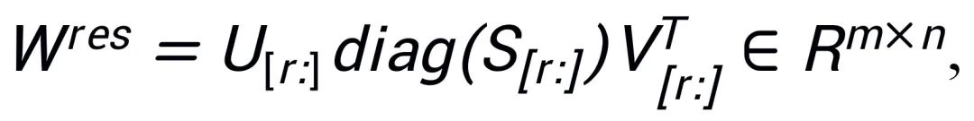
In contrast, PiSSA does not focus on △W but rather assumes that W possesses a very low intrinsic rank r. Therefore, it directly performs singular value decomposition on W, decomposing it into principal components A, B, and a residual term, ensuring that.

Assuming the singular value decomposition of W is, A and B are initialized using the top r singular values and singular vectors after SVD decomposition:

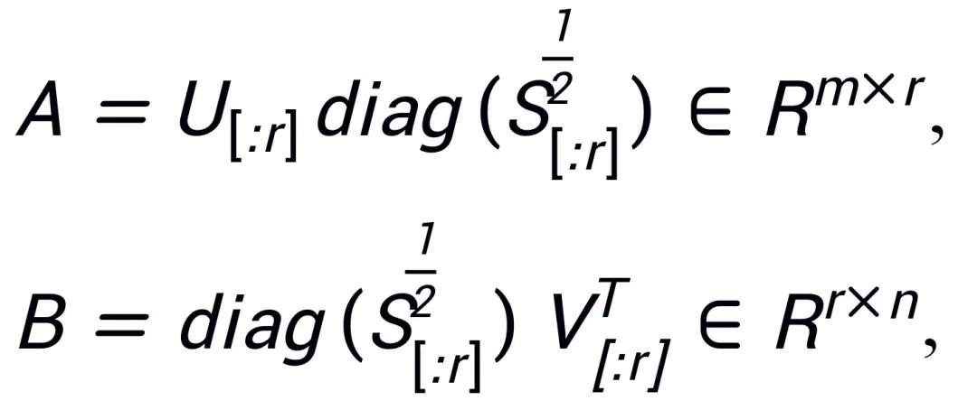
The residual matrix is initialized using the remaining singular values and singular vectors:

PiSSA directly fine-tunes the low-rank principal components A and B of W while freezing the less significant correction terms. Compared to LoRA, which initializes adapter parameters with Gaussian noise and 0 and freezes core model parameters, PiSSA converges faster and yields better results.

The pronunciation of PiSSA is similar to “pizza” – if the entire large model is likened to a complete pizza, PiSSA cuts off a corner, specifically the most filling corner (principal singular values and singular vectors), and re-bakes it (fine-tuning on downstream tasks) to the desired flavor.

Since PiSSA adopts the same architecture as LoRA, it can serve as an optional initialization method for LoRA, easily modified and called within the peft package (as shown in the code below).

The same architecture also allows PiSSA to inherit most of LoRA’s advantages, such as: using 4-bit quantization [3] for the residual model to reduce training costs; after fine-tuning, the adapter can be merged into the residual model without altering the model architecture during inference; there is no need to share complete model parameters, only a small number of PiSSA modules need to be shared, allowing users to load the PiSSA module directly to automatically perform singular value decomposition and assignment; a model can simultaneously use multiple PiSSA modules, etc. Some improvements to the LoRA method can also be combined with PiSSA, such as not fixing the rank of each layer and finding the optimal rank through learning [4]; using PiSSA-guided updates [5], thus breaking the rank limitation, etc.

Comparative Experiment on Fine-Tuning Effects of High, Medium, and Low Singular Values

To verify the impact of using different sizes of singular values and singular vectors to initialize the adapter on the model, the researchers used high, medium, and low singular values to initialize the adapters for LLaMA 2-7B, Mistral-7B-v0.1, and Gemma-7B, and then fine-tuned on the MetaMathQA dataset. The experimental results are shown in Figure 3. From the figure, it can be seen that the method using the primary singular values for initialization results in the lowest training loss and higher accuracy on the GSM8K and MATH validation sets. This phenomenon validates the effectiveness of fine-tuning the primary singular values and singular vectors.

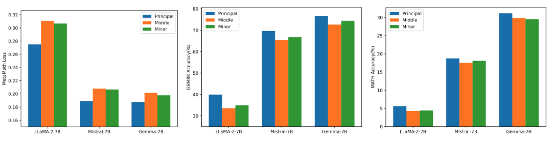
▲ Figure 3) From left to right are training loss, accuracy on GSM8K, and accuracy on MATH. Blue represents the maximum singular value, orange represents the medium singular value, and green represents the minimum singular value.

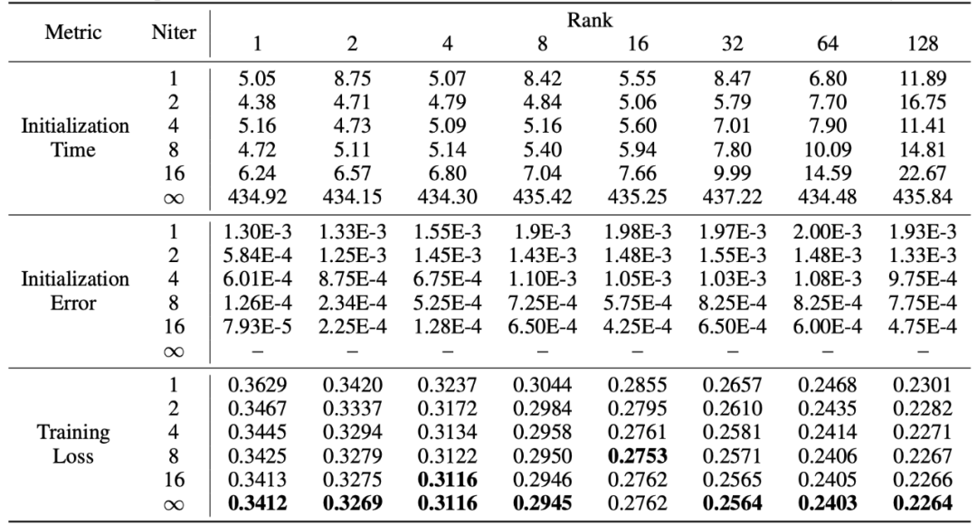
Fast Singular Value Decomposition

PiSSA inherits the advantages of LoRA, being user-friendly and outperforming LoRA. The trade-off is that during the initialization phase, the model needs to undergo singular value decomposition. Although it only requires decomposition once during initialization, it may still take several minutes or even tens of minutes.

Therefore, the researchers used a fast singular value decomposition [6] method to replace the standard SVD decomposition. The experiments in the table below demonstrate that it can achieve training set fitting results close to standard SVD decomposition in just a few seconds. Here, Niter indicates the number of iterations; the larger the Niter, the longer the time but the smaller the error. Niter = ∞ indicates standard SVD. The average error in the table represents the average L_1 distance between A and B obtained from fast singular value decomposition and standard SVD.

This work performs singular value decomposition on the weights of pre-trained models, using the most important parameters to initialize an adapter called PiSSA, and fine-tuning this adapter to approximate the effects of fine-tuning the complete model. Experiments indicate that PiSSA converges faster and yields better final results than LoRA, with the only cost being a few seconds of SVD initialization process.

So, would you be willing to spend a few more seconds for better training results by changing LoRA’s initialization to PiSSA with just one click?

References

[1] LoRA: Low-Rank Adaptation of Large Language Models

[2] Intrinsic Dimensionality Explains the Effectiveness of Language Model Fine-Tuning

[3] QLoRA: Efficient Finetuning of Quantized LLMs

[4] AdaLoRA: Adaptive Budget Allocation for Parameter-Efficient Fine-Tuning

[5] Delta-LoRA: Fine-Tuning High-Rank Parameters with the Delta of Low-Rank Matrices

[6] Finding structure with randomness: Probabilistic algorithms for constructing approximate matrix decompositions