Robust Pricing Research for Microgrids Considering Source-Load Imbalance

Main Content

In response to the issue of generation-consumption imbalance caused by a high proportion of renewable energy integration (such as significant fluctuations in wind and solar power generation, and difficulties in matching supply and demand), this program reproduces the study “Energy Imbalance Management Using a Robust Pricing Scheme“, innovatively proposing arobust dynamic pricing strategy that considers source-load imbalance. The program is written in MATLAB, with clear comments for research and learning purposes. The core principle is to intelligently adjust supply and demand throughreal-time electricity price signals:

1. Price Leverage Effect

• When electricity prices rise:⚡️ Generation side (such as thermal power/storage) increases production because the marginal cost is lower than the electricity price, whilethe consumption side reduces load actively because the electricity cost exceeds the marginal benefit.

• When electricity prices fall:⚡️ Renewable energy generation gainsabsorption space💡 Flexible loads such as electric vehicles/smart homes take the opportunity to consume electricity.

• ✅ Three-Dimensional Perception: Synchronously monitors generation, consumption, and storage status.

• ✅ Robust Decision-Making: Learns the fluctuation patterns of renewable energy (e.g., sudden changes in wind speed) using fuzzy rules.

• ✅ Rapid Balancing: Calculates optimal electricity prices in real-time using linear matrix inequalities.

• ✅ Innovative Method: Integrates fuzzy rule interpolation with H∞ robust control technology, designing dynamic pricing strategies by solving linear matrix inequalities.

• ✅ Core Advantages: Constructs a multi-dimensional fuzzy rule library to handle uncertainty, guiding the system to quickly restore balance through an active price fluctuation mechanism, providing an efficient market regulation tool for new power systems.

Partial Code

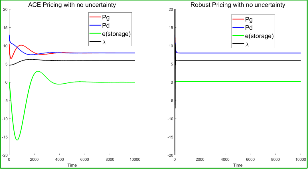
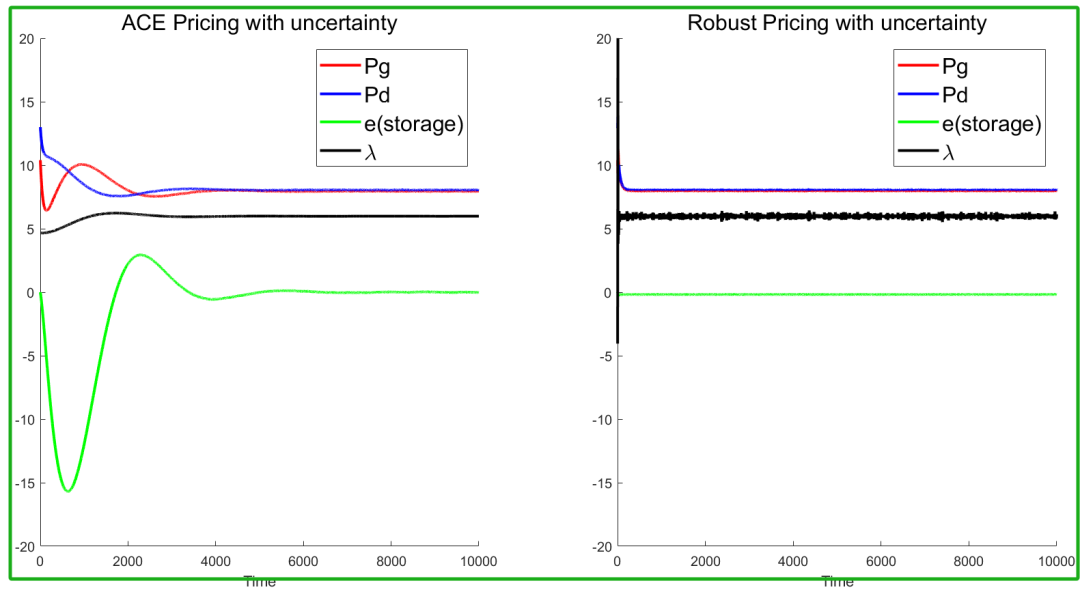
gamma = 10;  % Set the decay level γ in the H∞ performance index, a larger value indicates stronger robustness to uncertaintyfind = [0 0];  % Initialize flag variable (not used here)options = zeros(1,5);      % Configure LMI solver optionsoptions(2) = 200;          % Set maximum iteration count to 200options(3) = 500;          % Set feasibility precision requirement (smaller value means higher precision)options(5) = 1;            % Enable feasibility detection mode (1=enabled)setlmis([])                % Initialize LMI system% Define matrix variables (Lyapunov function candidate matrix)[Q, xa, xb] = lmivar(2, [3 3]);  % Type 2: 3x3 ordinary matrix (non-symmetric)% Define auxiliary matrix variable for controller gain[ym, ya, yb] = lmivar(2, [1 3]); % Type 2: 1x3 row vector (corresponding to K_m)% Construct LMI#1: Stability and H∞ performance conditions (corresponding to equation 25 in the paper)lmiterm([1 1 1 Q], Am(:, :, i), 1, 's');  % A_m*Q + Q*A_m^T ('s' indicates symmetric form)lmiterm([1 1 1 ym], tau, 1, 's');         % τ*y_m + y_m^T*τ^T (price feedback term)lmiterm([1 1 2 0], B);                    % B matrix (uncertainty input coefficient)lmiterm([1 1 3 Q], 1, C');                % Q*C^T (output weighting term)lmiterm([1 1 3 -ym], 1, D');              % -y_m*D^T (control output coupling term)lmiterm([1 2 2 0], -gamma*eye(3));        % -γI (H∞ performance diagonal term)lmiterm([1 2 3 0], zeros(3, 2));          % Zero matrix paddinglmiterm([1 3 3 0], -eye(2));              % -I (output performance weight)% Construct LMI#2: Lyapunov matrix positive definiteness constraint (Q > 0)lmiterm([-2 1 1 Q], 1, 1);  % -(-Q) = Q > 0 (negative sign indicates the left side of the inequality)% Complete LMI system descriptionlmis = getlmis;% Solve LMI feasibility problem[tmin, xfeas] = feasp(lmis, options);% Extract solution of Lyapunov matrix Q (9 elements corresponding to 3x3 matrix)Q = [xfeas([1 2 3])'; xfeas([4 5 6])'; xfeas([7 8 9])'];% Extract solution of auxiliary matrix y_m (3 elements corresponding to 1x3 vector)Ym(:, :, i) = xfeas([10:12])';% Calculate controller gain matrix K_m = y_m * Q^{-1}Km(:, :, i) = Ym(:, :, i)/Q;% Record performance index and solution state of the current subsystemgamma_list(i) = gamma;  % Store the used γ valuet_list(i) = tmin;       % Store the solution result

Results Overview

“Read the Original Text” to obtain the program source code

Scan or Read the Original Text to jump to the program page:

Want to learn more about the program? Follow the tutorial below to view the program directory!