
Click the blue text above to follow us

📋📋📋 The content of this article is as follows: 🎁🎁🎁
Directory
💥1 Overview
📚2 Results
2.1 Stationary Signal
2.2 Noisy Non-Stationary Signal
2.3 Signal with Closed Modes
🎉3 References
🌈4 Matlab Code Implementation



1 Overview
This article explains a data-driven time-varying AM-FM signal adaptive signal decomposition method, data-driven adaptive linear frequency modulation mode decomposition, and its application in non-stationary conditions for machine fault diagnosis, mechanical systems and signal processing, adaptive linear frequency modulation mode tracking: algorithms and applications, nonlinear linear frequency modulation mode decomposition: a variational method.

Reproducing some results from the paper: Hongbing Wang, Shiqian Chen, et al. Data-driven adaptive chirp mode decomposition with application to machine fault diagnosis under non-stationary conditions, Mechanical Systems and Signal Processing, 2022. The algorithm used in the paper is an improved version of that in the paper: Shiqian Chen, et al. Adaptive chirp mode pursuit: Algorithm and applications, Mechanical Systems and Signal Processing, 2018. Some of the scripts are adopted from the paper: Shiqian Chen, et al. Nonlinear Chirp Mode Decomposition: A Variational Method, IEEE Transactions on Signal Processing, 2017. and the paper: Shiqian Chen, et al. Detection of rub-impact fault for rotor-stator systems: A novel method based on adaptive chirp mode decomposition, Journal of Sound and Vibration, 2019.


2 Results
 2.1 Stationary Signal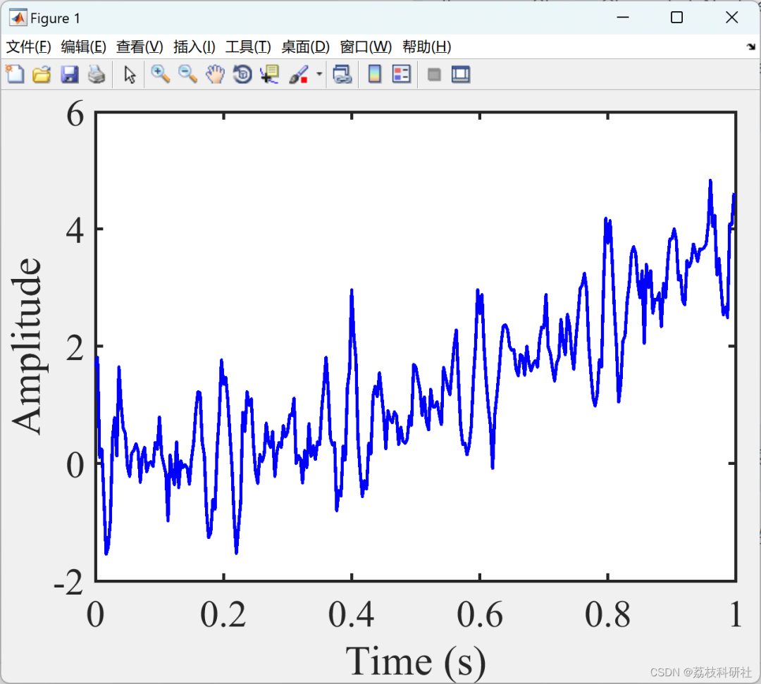
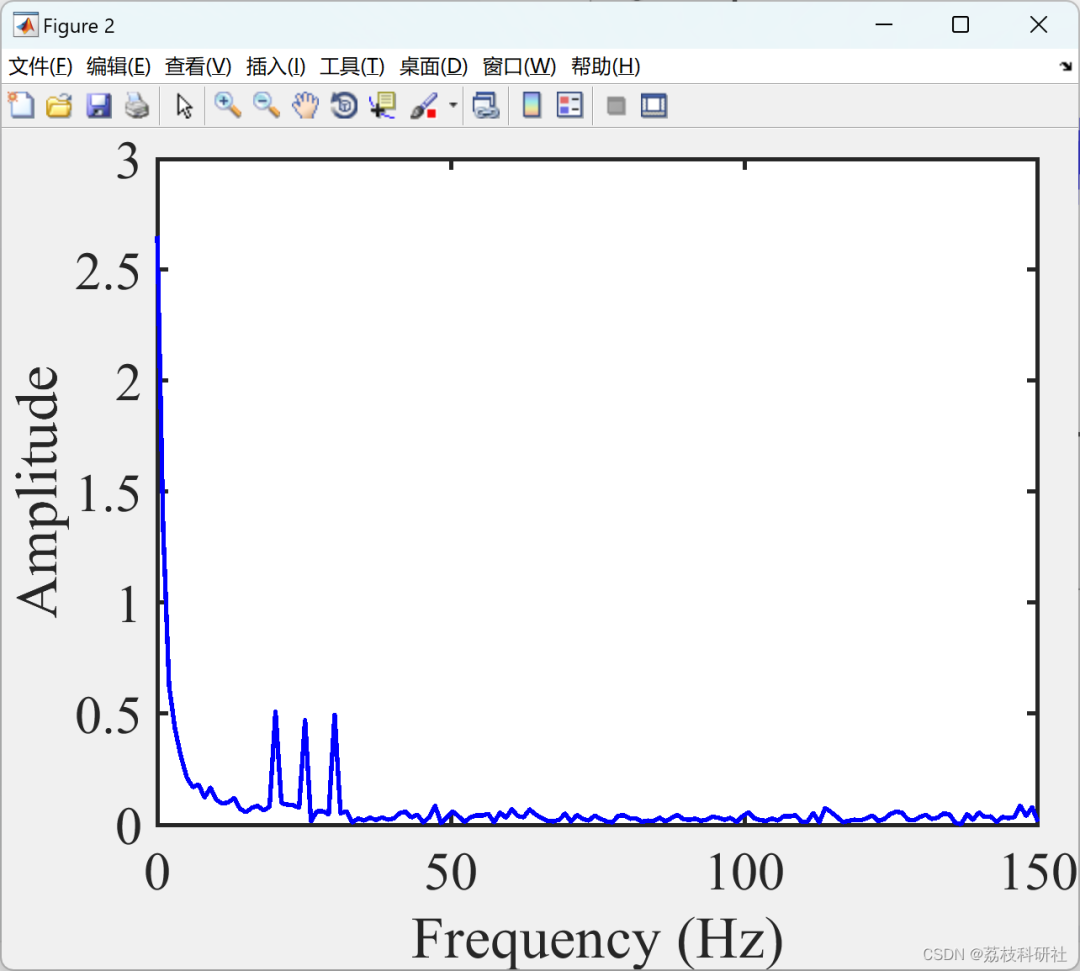
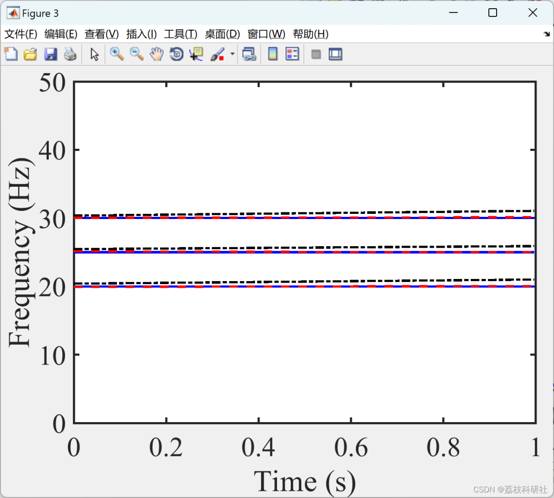
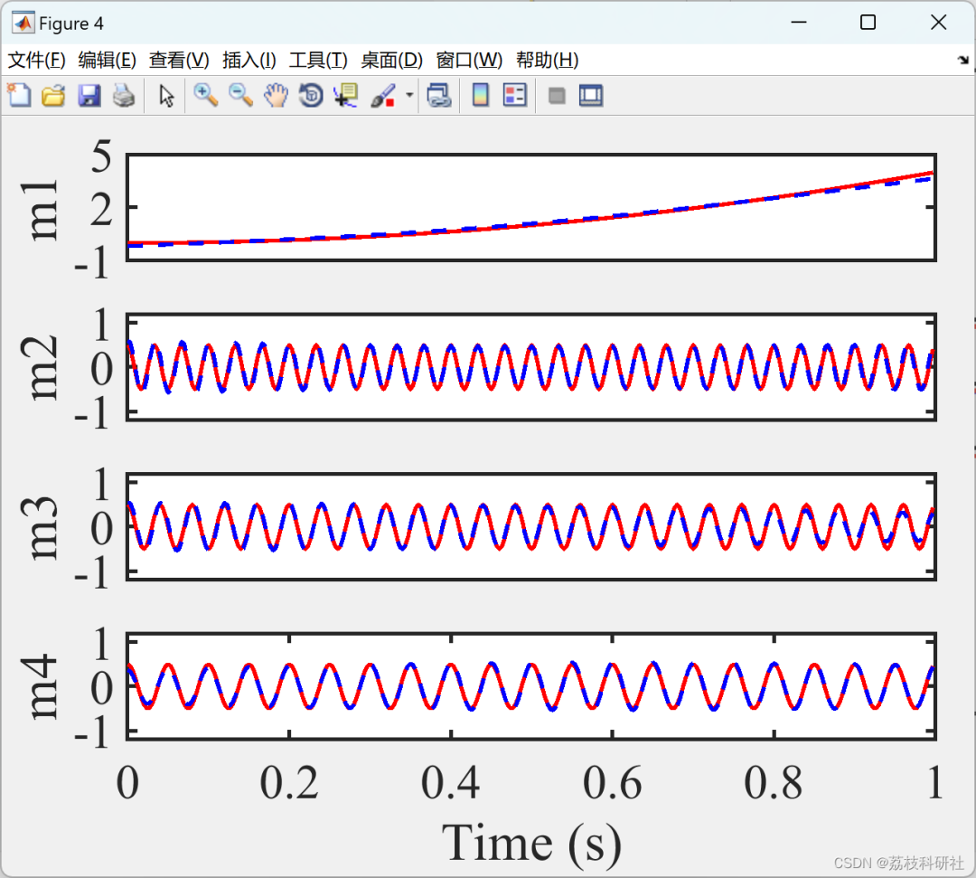
 2.2 Noisy Non-Stationary Signal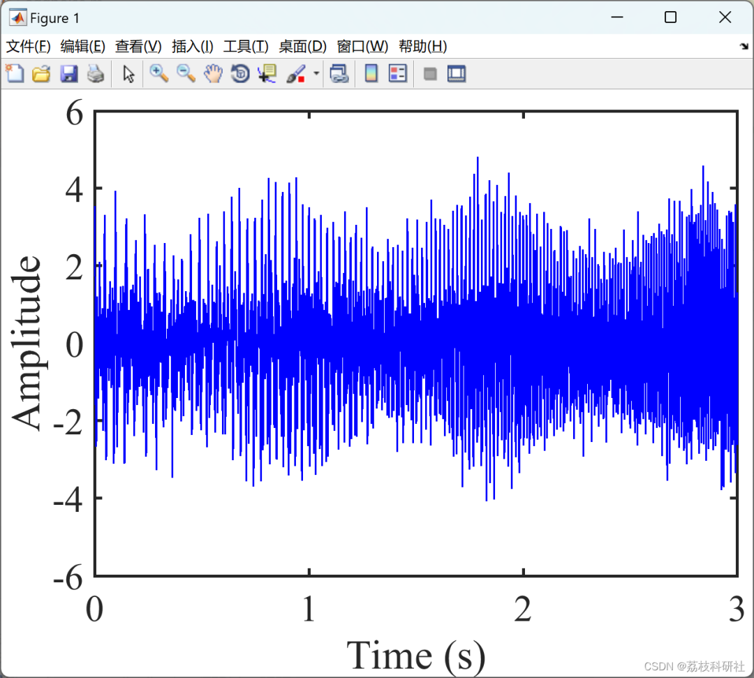

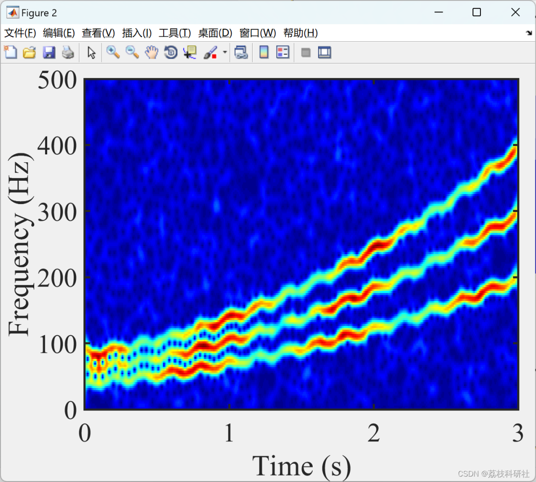
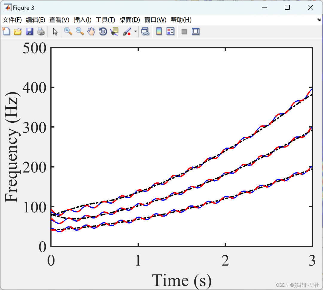
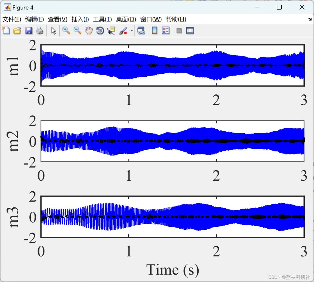
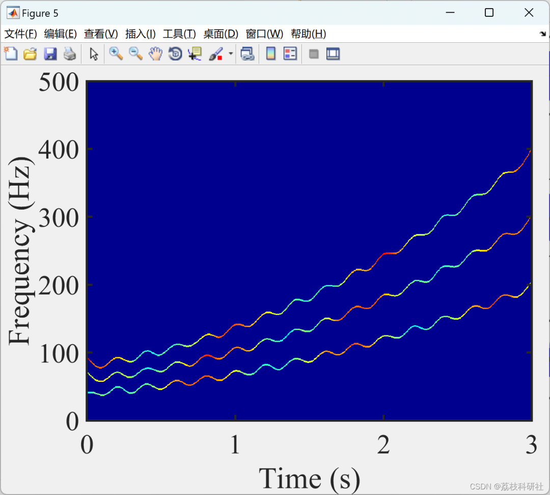
 2.3 Signal with Closed Modes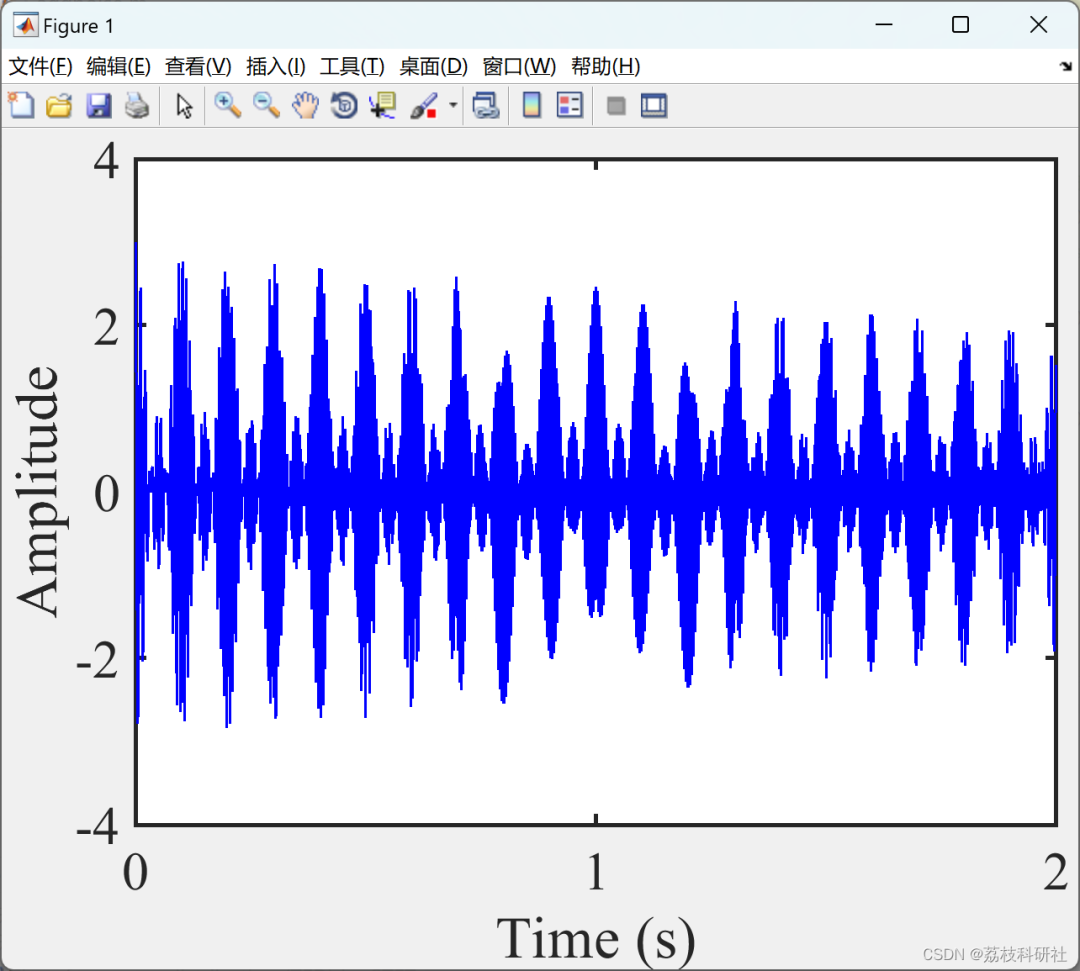
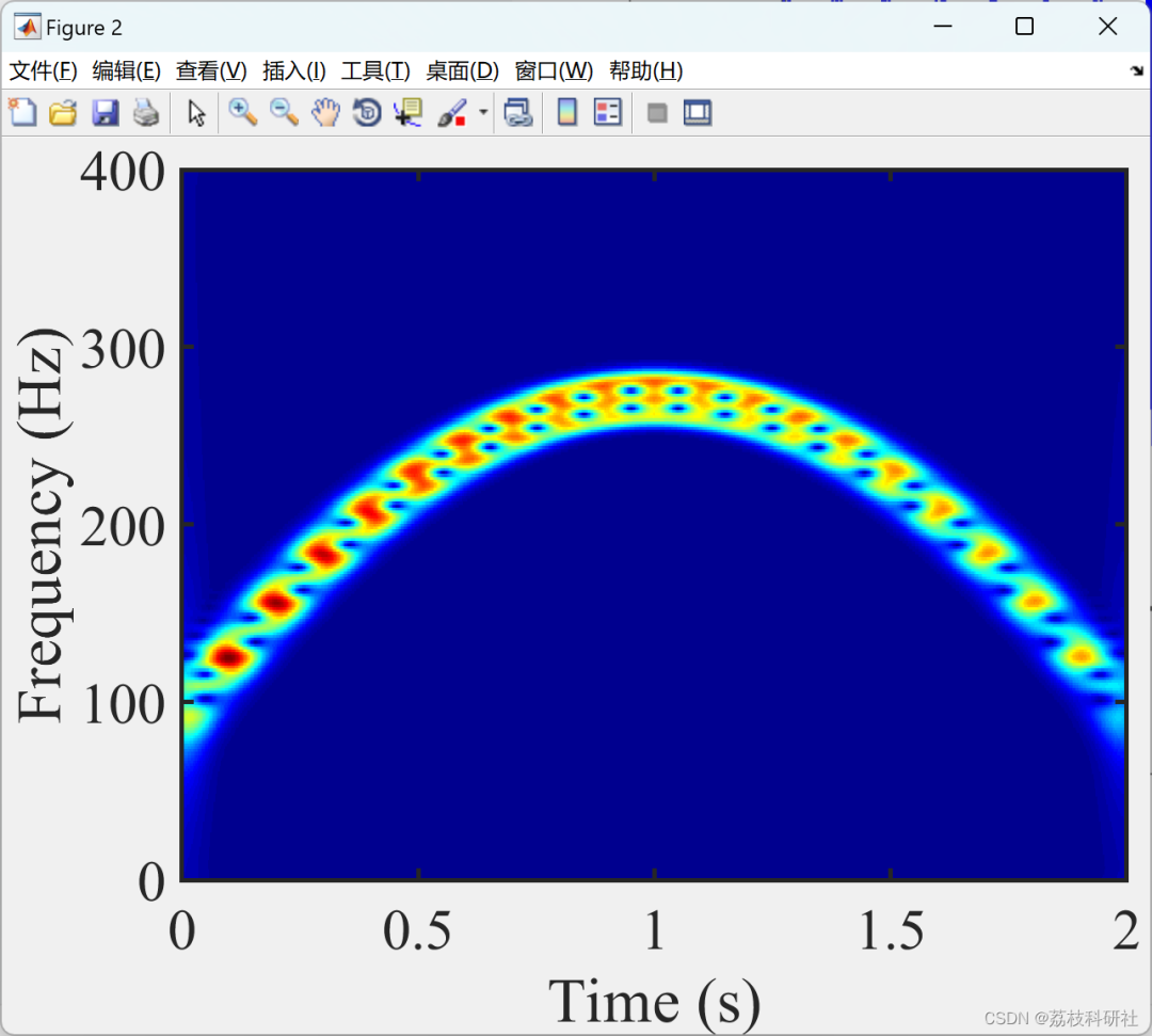
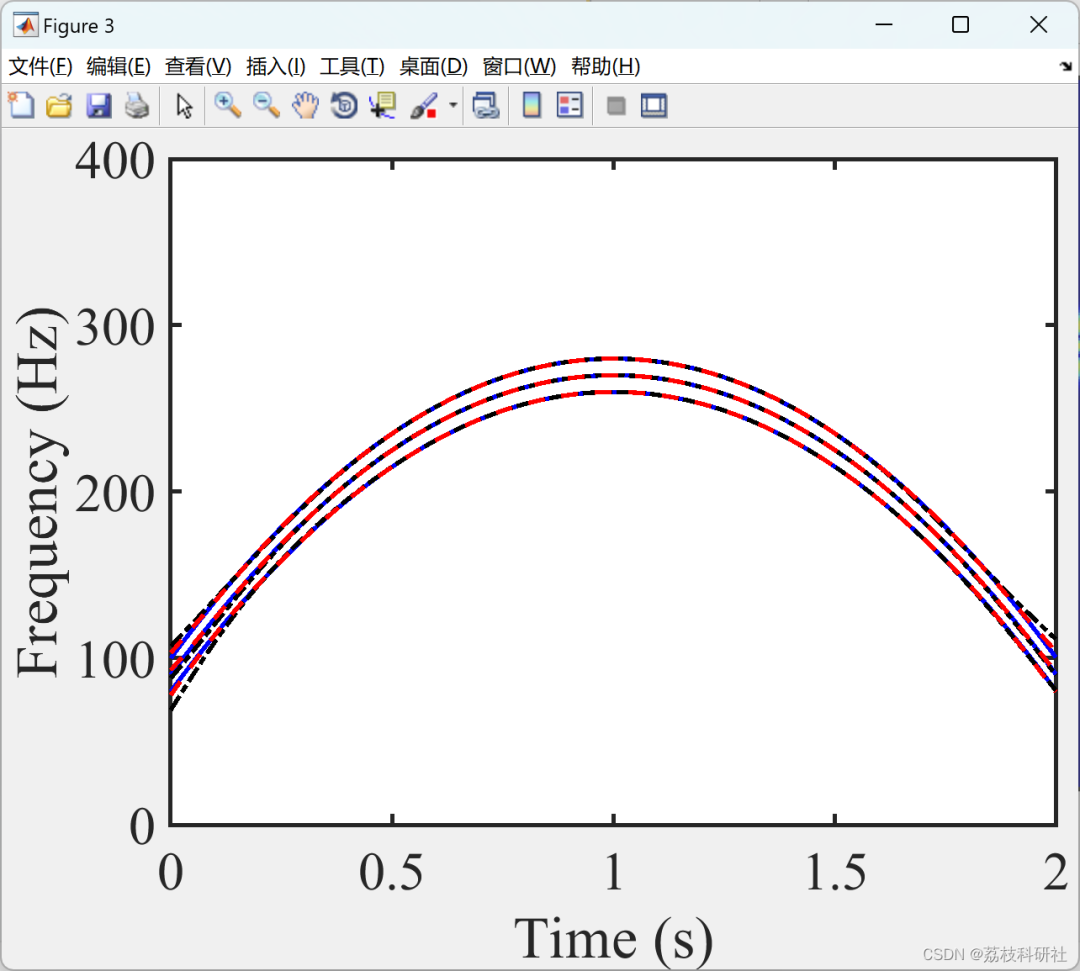
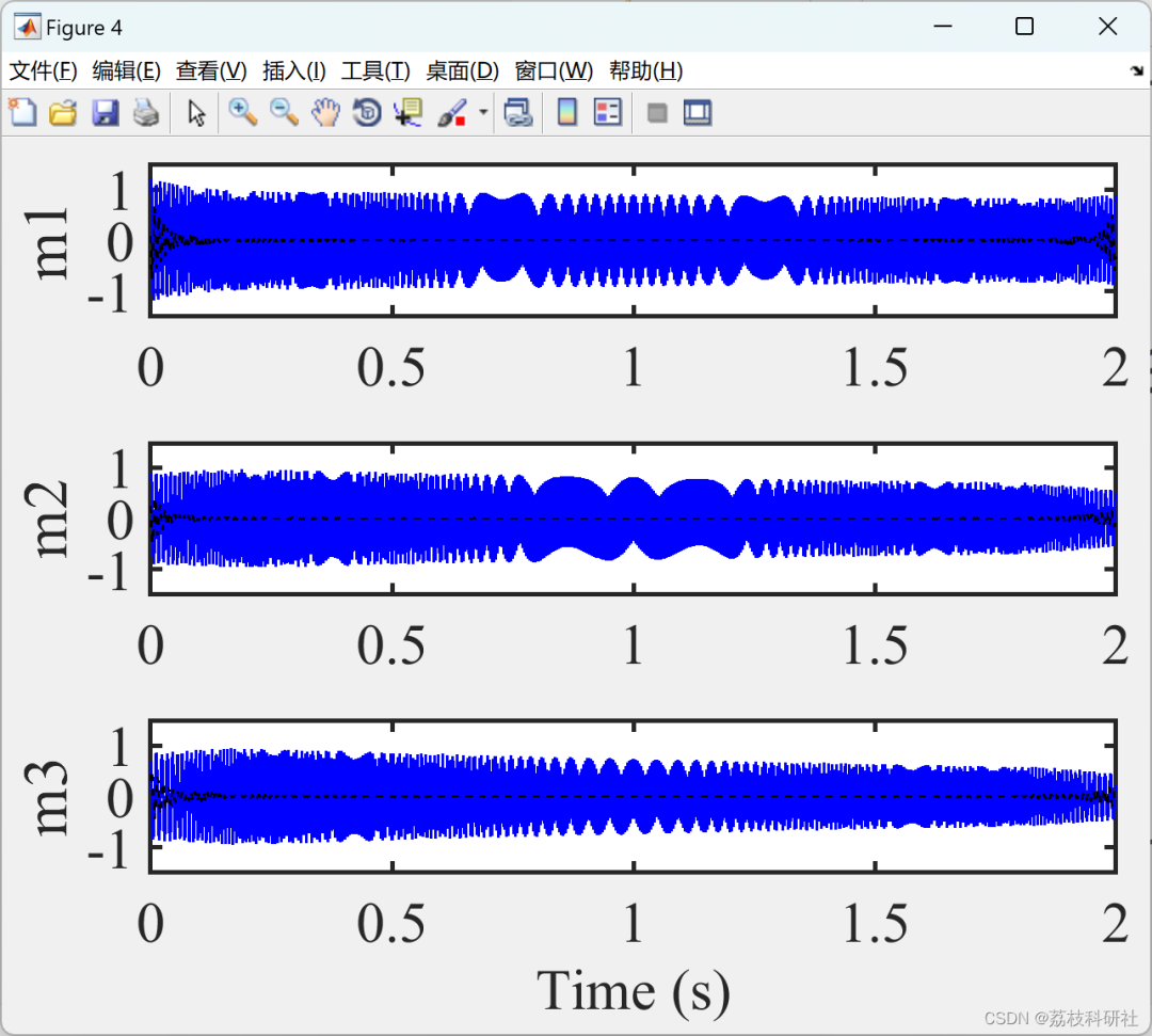
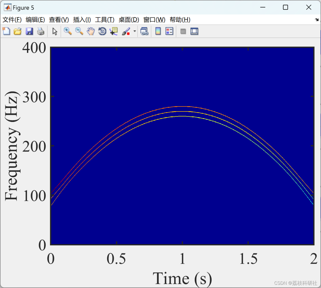
部分代码:%%%%%%%%% Signal withClose modes %%%%%%%%%clc;clear;closeall;SampFreq =800;t =0:1/SampFreq:2-1/SampFreq;a1 =exp(-0.1*t); % Instantaneous amplitude (IA) 1Sig1 = a1.*cos(2*pi*(-60*t.^3+180*t.^2+100*t)); % mode 1IF1 =-180*t.^2+360*t+100;% instantaneous frequency (IF) 1a2 =exp(-0.2*t);% IA 2Sig2 = a2.*cos(2*pi*(-60*t.^3+180*t.^2+90*t)); % mode 2IF2 =-180*t.^2+360*t+90;% IF2a3 =exp(-0.3*t);% IA 3Sig3 = a3.*cos(2*pi*(-60*t.^3+180*t.^2+80*t)); % mode 3IF3 =-180*t.^2+360*t+80;% IF3Sig = Sig1 + Sig2 + Sig3;noise = addnoise(length(Sig),0,0);Sign = Sig+noise; figureset(gcf,'Position',[20100640500]);plot(t,Sign,'b-','linewidth',1);axis([02-44]);set(gca,'xtick',[0:1:2]);set(gca,'ytick',[-4:2:4]);xlabel('Time (s)','FontSize',24);ylabel('Amplitude','FontSize',24);set(gca,'FontSize',24,'FontName','Times New Roman','linewidth',2);set(gca,'looseInset',[0.020.020.020.02])%%Time-frequency distribution (TFD) by STFTfigure[Spec,f] = STFT(Sign',SampFreq,512,218);imagesc(t,f,abs(Spec)); set(gcf,'Position',[20 100 640 500]); axis([0 2 0 400]);xlabel('Time (s)','FontSize',24);ylabel('Frequency (Hz)','FontSize',24);set(gca,'YDir','normal');set(gca,'looseInset',[0.02 0.02 0.02 0.02])set(gca,'FontSize',24,'FontName','Times New Roman','linewidth',2);colormap('jet')%% DDACMDtic[iniIF,eIF,eIA,IMF] = DDACMD(Sign,SampFreq);toc%% Estimated IFfigureset(gcf,'Position',[20 100 640 500]);plot(t,IF1,'b-',t,iniIF(1,:),'k-.',t,eIF(1,:),'r--','linewidth',2) holdonplot(t,IF2,'b-',t,iniIF(2,:),'k-.',t,eIF(2,:),'r--','linewidth',2)holdonplot(t,IF3,'b-',t,iniIF(3,:),'k-.',t,eIF(3,:),'r--','linewidth',2) xlabel('Time (s)','FontSize',24);ylabel('Frequency (Hz)','FontSize',24);set(gca,'FontSize',24,'FontName','Times New Roman','linewidth',2);axis([020400]);set(gca,'looseInset',[0.020.020.020.02])%% Reconstructed modesfigureset(gcf,'Position',[20100640500]);axes('position',[0.130.800.840.17]);plot(t,IMF(1,:),'b-','linewidth',1);holdonplot(t,Sig1-IMF(1,:),'k--','MarkerIndices',1:60:length(t),'linewidth',1);axis([02-1.51.5]);set(gca,'xtick',[0:0.5:2]);set(gca,'ytick',[-101]);ylabel('m1','FontSize',24);set(gca,'FontSize',24,'FontName','Times New Roman','linewidth',2);axes('position',[0.130.490.840.17]);plot(t,IMF(2,:),'b-','linewidth',1);holdonplot(t,Sig2-IMF(2,:),'k--','MarkerIndices',1:60:length(t),'linewidth',1);axis([02-1.51.5]);set(gca,'xtick',[0:0.5:2]);set(gca,'ytick',[-101]);ylabel('m2','FontSize',24);set(gca,'FontSize',24,'FontName','Times New Roman','linewidth',2);axes('position',[0.130.180.840.17]);plot(t,IMF(3,:),'b-','linewidth',1);holdonplot(t,Sig3-IMF(3,:),'k--','MarkerIndices',1:60:length(t),'linewidth',1);axis([02-1.51.5]);set(gca,'xtick',[0:0.5:2]);set(gca,'ytick',[-101]);ylabel('m3','FontSize',24);set(gca,'FontSize',24,'FontName','Times New Roman','linewidth',2);xlabel('Time (s)','FontSize',24);%% Adaptive time-frequency spectrumband = [0 SampFreq/2];[ASpec,fbin] = TFspec(eIF(1:3,:),eIA(1:3,:),band);figureimagesc(t,fbin,abs(ASpec)); set(gcf,'Position',[20100640500]); axis([020400]);xlabel('Time (s)','FontSize',24);ylabel('Frequency (Hz)','FontSize',24);set(gca,'YDir','normal');set(gca,'looseInset',[0.020.020.020.02])set(gca,'FontSize',24,'FontName','Times New Roman','linewidth',2);colormap('jet')
3References
Some theoretical sources are from the internet. If there is any infringement, please contact for removal.

[1] Shiqian Chen (2023). Data-driven adaptive linear frequency modulation mode decomposition.

4 Matlab Code Implementation
Previous Recommendations
Capacity optimization configuration of wind-solar-hydrogen microgrid based on non-cooperative game (Matlab code implementation)
Optimal scheduling of water and fire power considering a group of hydropower stations (Python code implementation)
[Nonlinear Linear Frequency Modulation Mode Decomposition] Group delay estimation and mode separation of dispersive signals with cross-signal modes (Matlab code implementation)
Prediction based on Bayesian optimization CNN-LSTM hybrid neural network (Matlab code implementation)
Research on blind modal identification based on Hankel matrix (BMIDHM) (Matlab code implementation)
Joint configuration method for distributed power and electric vehicle charging stations under unidirectional/bidirectional V2G environment (Matlab code implementation)
[Fault Diagnosis] Whale algorithm based on Von Neumann topology for fault diagnosis of rolling bearings (Matlab code implementation)
Research on optimal scheduling of cascade hydropower stations based on genetic algorithm (Python code implementation)
[Image Processing] Image region segmentation based on K-means clustering algorithm (Matlab code implementation)
[State Estimation] Algorithms for analysis, state estimation, and fault detection for descriptor LTI and LPV systems (Matlab code implementation)