0. Introduction
Official documentation for m_map (Chinese version):
https://pan.baidu.com/s/14CIblgcoy3MDKAmw3jO0qA?pwd=eaua Extraction code: eaua
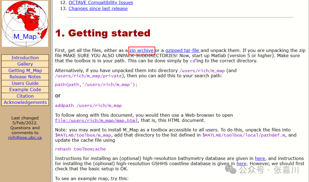
1. Downloading the m_map Toolkit
Method 1: Download from the official m_map website:
https://www-old.eoas.ubc.ca/~rich/mapug.html
Method 2: Download directly from the Baidu Cloud provided by the author:
https://pan.baidu.com/s/1aKhTfwzqM1qt8FgETuFPeA?pwd=eism Extraction code: eism
2. Downloading High-Precision Terrain and Coastline Data
The coastline and terrain data that comes with m_map is of low precision and often cannot meet actual task requirements. High-precision coastline and terrain data needs to be downloaded separately, as follows:
Step 1: Go to the NOAA website to download high-precision coastline data
https://www.ngdc.noaa.gov/mgg/shorelines/shorelines.html
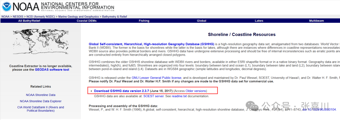
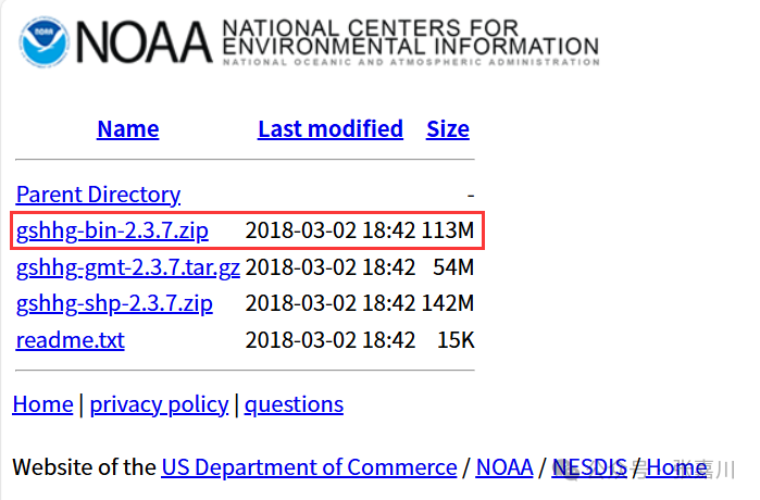
Step 2: Download the first *.zip file
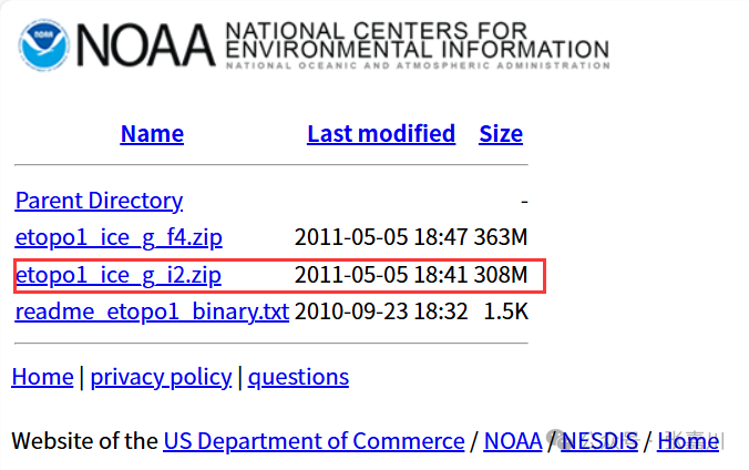
Step 3: Go to the NOAA website to download high-precision terrain data (recommended 16-bit integer, i.e., i2)
https://www.ngdc.noaa.gov/mgg/global/relief/ETOPO1/data/ice_surface/grid_registered/binary/
3. Configuring m_map, High-Precision Coastline, and Terrain File Paths
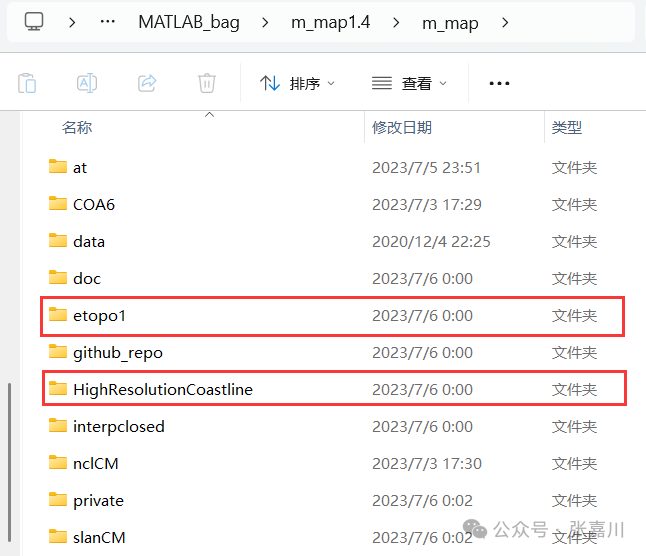
First, unzip the downloaded m_map folder and place it in a specific path.
Next, create folders named etopo1 and HighResolutionCoastline in the path where m_map is located to store terrain and coastline files, respectively.
Finally, unzip the high-precision terrain data downloaded from NOAA into the corresponding folders, for example:
4. Configuring the Paths for m_etopo2.m and m_gshhs.m
Modify the PATHNAME in the m_etopo2.m function to the newly created etopo1 folder in the path where m_map is located:
PATHNAME='E:\1. MATLAB\MATLAB_bag\m_map1.4\m_map\etopo1/'; Modify the PATHNAME in the m_gshhs.m function to the newly created HighResolutionCoastline folder in the path where m_map is located:
FILNAME='HighResolutionCoastline/';At this point, the m_map related environment configuration is complete.
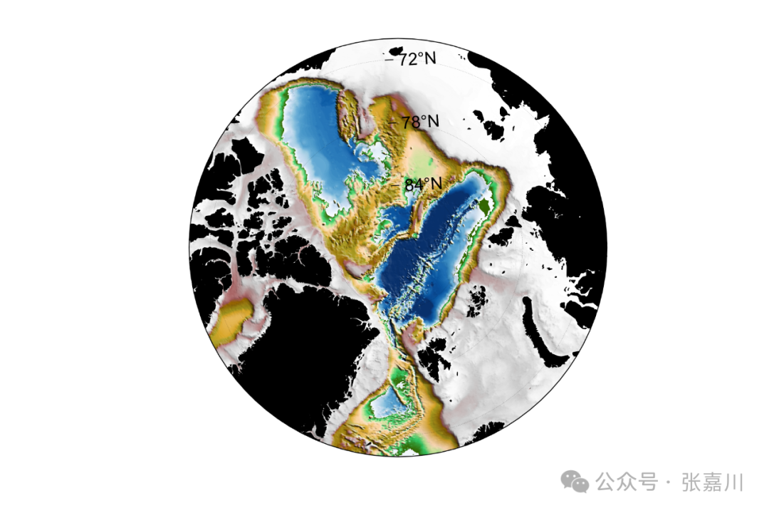
5. Example of High-Precision Terrain and Coastline Mapping
%% Polar Projection High-Precision demo02 = figure(2)% Mainly using m_etopo2 function and m_gshhs functionset(demo02,'position',[700,50,600,400])% Set figure window sizem_proj('stereographic','lat',90,'1ong',10,'radius',20);caxis([-4000 0]) colormap([m_colmap('blue',50);m_colmap('gland',200)])% Combine colorbarm_etopo2('shadedrelief','lightangle',45);% Terrain data m_gshhs('lc','patch',[0 0 0],'Edgecolor','k');% Coastline data% m_gshhs first parameter: c, l, i, h, f represent coarse/low/medium/high/full resolution% m_gshhs second parameter: c, b, r represent coastline, national borders, and rivershc=colorbar;set(get(hc,'title'),'string','Elevation(m)') % Add title to colorbara=get(hc, 'Position') ;% Get the lower left x,y coordinates of colorbar, as well as width and height.set(hc, 'Position', [a(1)+0.05,a(2),0.7*a(3),a(4)]) % Modify colorbar positionm_grid('xtick',[],'tickdir','in', 'ytick',4,' linest',':','xaxisloc','top');title('Temperature','fontsize',12)print(demo02,'d:/桌面/demo01','-dpng','-r600')% Save high-precision image with dpi=600