Logistics Center Location Based on Sparrow Algorithm
Abstract: This article mainly introduces the logistics center location algorithm based on the Sparrow algorithm.
1. Logistics Center Location Model
The logistics center, as the core node of the logistics network, has a crucial impact on the efficiency, cost, and service level of the entire supply chain. A reasonable logistics center location can effectively reduce transportation costs, shorten delivery times, and improve response speed, thereby enhancing the market competitiveness of enterprises. However, the logistics center location is a complex decision-making problem that involves various factors such as geographical location, transportation, market demand, land costs, and policies, making it a typical NP-hard problem. Traditional optimization methods often face limitations such as computational complexity and the tendency to fall into local optima when solving large-scale, multi-constraint logistics center location problems. Therefore, seeking efficient and robust optimization algorithms to enhance the scientific and rational aspects of logistics center location has become a key issue that needs to be addressed in the logistics field.
First, it is necessary to perform mathematical modeling of the logistics center location problem. Depending on different application scenarios and requirements, different models can be selected. This article will adopt the classic Capacitated Facility Location Problem (CFLP) as the research object. CFLP aims to select a portion of candidate logistics center locations to meet customer demand while minimizing total costs and adhering to the capacity constraints of each logistics center.
Objective Function
Objective Function: Minimize Constraints: (Ensure that each customer’s demand can only be met by one logistics center) (Ensure that the total demand of each logistics center does not exceed its capacity) (Service can only be provided to customers if the logistics center is selected) (Decision variable indicating whether customer i is served by logistics center j) (Decision variable indicating whether logistics center j is selected)Where:
- • i represents the customer number,
- • j represents the candidate logistics center number,
- • represents the transportation cost from customer to logistics center
- • represents the fixed cost of logistics center
- • represents the variable cost of logistics center
- • represents the demand of customer i
- • represents the capacity of logistics center
- • indicates whether the demand of customer i is met by logistics center j, taking values of 0 or 1
- • indicates whether logistics center is selected, taking values of 0 or 1
- • is the weight coefficient of each cost in the total cost
The goal of this model is to minimize total costs, including transportation costs and fixed costs. The constraints ensure that each customer’s demand is met, the total demand of each logistics center does not exceed its capacity, and only selected logistics centers can provide services to customers.
2. Sparrow Algorithm
For the principle of the Sparrow algorithm, please refer to: https://blog.csdn.net/u011835903/article/details/108830958
3. Experimental Case
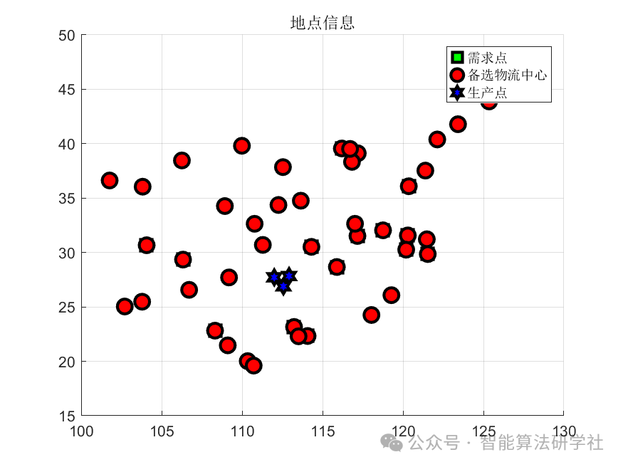
This article selects a logistics center case, with specific information as follows:
Node Latitude and Longitude Information:
| Node | Longitude | Latitude | Type | Fixed Cost |
| Nanjing | 118.76 | 32.04 | 1 | 260 |
| Wuxi | 120.3 | 31.57 | 1 | 225 |
| Hefei | 117.17 | 31.52 | 1 | 225 |
| … | … | … | … | … |
Where type 3 is the production site, type 1 is the alternative logistics center, and types 1+2 are demand locations.
Distance from Logistics Nodes to Production Sites:
| Unit: meters | Xiangtan | loudi | Hengyang |
| Nanjing | 793268 | 844115 | 894681 |
| Wuxi | 896726 | 964106 | 1014672 |
| Hefei | 674753 | 721492 | 772059 |
| … | … | … | … |
Distance from Logistics Nodes to Demand Points:
| Unit: kilometers | Nanjing | Wuxi | Hefei | Hangzhou | Ningbo | Guangzhou | Shenzhen | Nanning | Wuhan | Nanchang | Beijing | Chengdu | Chongqing | Qingdao |
| Nanjing | 0 | 145 | 139 | 235 | 359 | 1143 | 1164 | 1468 | 446 | 536 | 851 | 1393 | 1215 | 477.4 |
| Wuxi | 144 | 0 | 280 | 177 | 225 | 1221 | 1241 | 1586 | 587 | 611 | 933 | 1534 | 1356 | 534.5 |
| Hefei | 138 | 280 | 0 | 354 | 480 | 1018 | 1046 | 1343 | 321 | 396 | 855 | 1268 | 1090 | 593.9 |
| … | … | … | … | … | … | … | … | … | … | … | … | … | … | … |
Demand:
| Unit: ten thousand tons | Xianggang | Lian Steel | Heng Steel | Total |
| Nanjing | 47 | 10 | 8 | 65 |
| Wuxi | 0 | 15 | 25 | 40 |
| Hefei | 15 | 28 | 5 | 48 |
| … | … | … | … | … |
4. Experimental Results


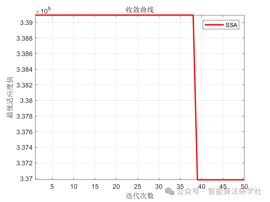
5. Matlab Code
Get it through “Read the original text“