Skip to content
An oscilloscope is a primary instrument for time-domain measurements. Currently, most digital oscilloscopes include approximately 25 built-in measurement parameters as standard supplements. By adding application customization options, the number of parameters can be increased to over a hundred. Even with such a vast measurement capability, some measurements must utilize existing measurement tools to derive results. One of these is the measurement of the time constant of an exponential signal.
Many physical phenomena are related to the charging and discharging of energy storage devices such as capacitors and inductors, resulting in waveforms with exponential rise or fall edges, where the exponential time constant reveals information about the fundamental processes and component values. Being able to measure the exponential time constant using an oscilloscope is useful for better understanding circuit operation. However, oscilloscopes do not directly provide measurement parameters for the exponential time constant. This article will demonstrate how to achieve the measurement of the exponential time constant through manual cursor measurements, as well as utilizing the oscilloscope’s signal processing and built-in measurement functions to directly read the time constant. Let’s start by reviewing exponential signals.
A typical exponential process can be defined by either of the following equations, depending on the slope of the exponential:
Exponential Rise: V(t)=1–a*e^(-t/τ)+b
Exponential Decay: V(t)=a*e^(-t/τ)+b
V(t) is the voltage changing over time, in V;
a and b are arbitrary constants;
τ is the exponential time constant, in s;
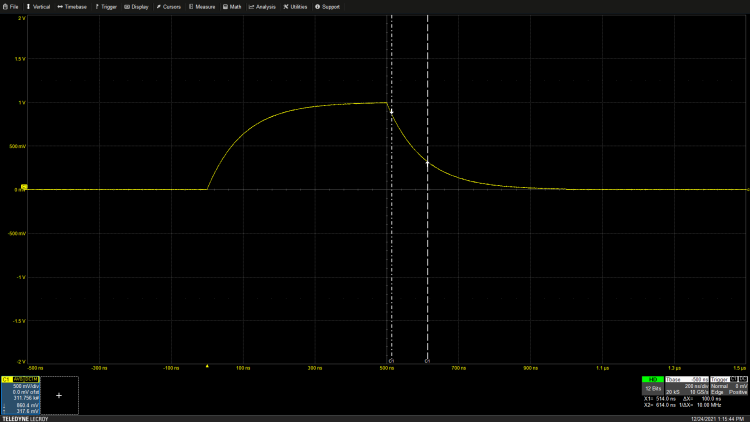
Figure 1 is an example of an exponential pulse, showing the rise and fall edges captured on the oscilloscope. The exponential constants in this example are a=1 and b=0. To improve the signal-to-noise ratio and increase measurement accuracy, the waveform has been averaged.
Figure 1: Measuring the time constant of an exponential pulse decay using the oscilloscope’s cursor.
Considering the exponential decay equation, for constants a=1 and b=0, when time t equals the time constant τ, the voltage value equals 1/e or 0.368. This is key to measuring the time constant on the oscilloscope. By setting the cursor to measure the amplitude variation at 0.368 times constant a, the time difference between the cursors is the time constant. In the example, the amplitude value read by the left cursor is 860.4 mV. Adjust the right cursor until its amplitude reading is as close as possible to 36.8% of that value, which in this case is 317.6 mV. The indicated time difference between the cursors is 100ns, which is the time constant τ for the decay edge.
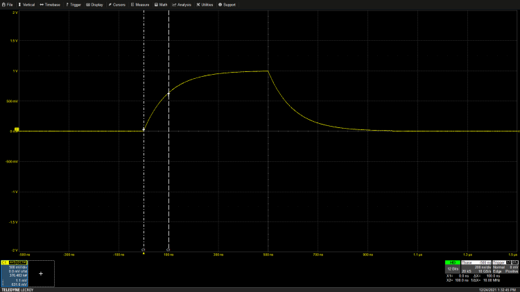
Similarly, the time constant for the rise edge can also be determined as shown in Figure 2.
Figure 2: Measuring the time constant of the exponential pulse rise edge.
From the rise edge equation, the voltage value at one time constant from the start is 1-0.368 or 0.632 of the maximum value. For a 1V peak signal, set the cursor again to measure the amplitude difference at 0.632V above zero, at which point the time constant is 100ns. This method employs traditional techniques and can be performed on any oscilloscope, yielding reasonable results, but it does require extensive setup. Accuracy depends on the user’s ability to correctly set the cursors. If possible, it is best to utilize the oscilloscope’s measurement parameters for the most accurate results.
If the oscilloscope’s available mathematical operations include the natural logarithm function, and its measurement parameters include slope or slew rate measurements, the time constant can be read directly.
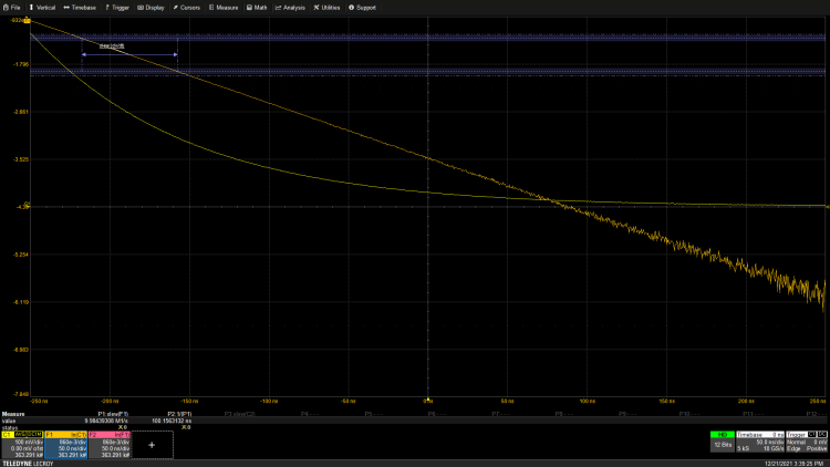
Taking the natural logarithm of the exponential function results in a linear function, whose slope equals the exponential time constant, as shown in Figure 3.
Figure 3: The natural logarithm of the exponential function is a straight line with a slope proportional to the exponential time constant.
The natural logarithm of the captured signal produces a straight line, which is a good test to ensure that the acquired waveform is indeed exponential. If the natural logarithm of the taken signal is not a straight line, then the waveform is not exponential. The slope of the linear natural logarithm can be calculated by measuring the signal’s slew rate, which is the change in amplitude per unit time (ΔV/Δt), as shown in measurement parameter 1 in the figure. The result is 9.9965 MV/s. Note that slew rate measurements require the user to select the slope of the signal being measured; in this case, the signal has a negative slope. The time constant is the slope of the line, which is the reciprocal of the slew rate or (Δt/ΔV). This oscilloscope supports calculations using parameters including sum, difference, product, ratio, reciprocal, and scaling of parameters. The reciprocal of P1 is calculated in parameter P2, which, when applied to parameter P1, returns a negative slope of 100ns/V. This is precisely the time constant of the exponential waveform.
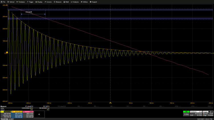
Exponential signals often manifest as modulation on high-frequency carriers, naturally occurring when the RF carrier is keyed on or off. Measuring the time constant of such signals requires extracting the modulated envelope, as shown in Figure 4.
Figure 4: Measuring the time constant of the carrier’s exponential amplitude modulation requires demodulating the modulated signal to extract the modulation envelope.
In this case, there is a decaying exponential amplitude modulation on a 100MHz carrier. The mathematical function F1 utilizes an optional demodulation function to extract the exponential modulation envelope displayed on the modulated signal. From this point, the natural logarithm function is applied to the exponential envelope, with the parameter reading the slope of the natural logarithm trajectory being the same as before. The result is exactly the time constant of 100ns.
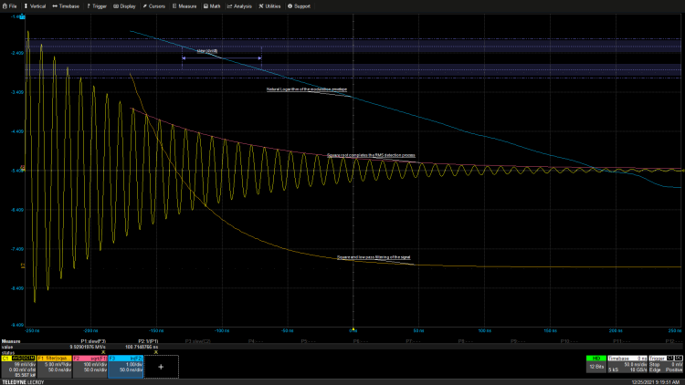
If the oscilloscope does not have demodulation capabilities, another demodulation technique is to perform RMS detection on the modulated carrier. This involves squaring the modulated carrier, filtering the squared function, and then taking the square root of the filtered function, as shown in Figure 5.
Figure 5: Measuring the time constant of the exponential modulated carrier using RMS measurement through squaring, filtering, and square root functions.
RMS demodulation is a traditional technique. The demodulated waveform will be truncated by the filtering operation, but this does not hinder the measurement of the exponential time constant. The time constant can be determined by calculating the reciprocal of the slew rate measurement and parameter mathematics.
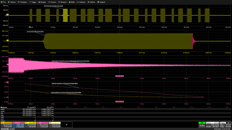
Figure 6 provides a practical example of measuring the time constant of the RF pulse train in a remote control door lock fob signal. The remote control door lock fob generates an encoded signal using a carrier frequency of 390 MHz.
Figure 6: Measuring the exponential decay time constant of the RF signal pulse from the remote control door lock transmitter.
The remote key generates 21 different widths of RF pulses, as shown in the top trace. Considering EMI factors, it is often required to control RF keying through limited attack and decay times to minimize spectral “splash” caused by fast on/off keying. In the closely adjacent trace below, the fifth pulse has been horizontally expanded using the trace scaler. The leading and trailing edges of the pulse exhibit exponential characteristics. This trace has been further expanded into the third trace below to show the entire decay amplitude. The demodulation function is used to extract the exponential envelope, as shown in the bottom trace. The natural logarithm of the modulation envelope is closely adjacent to this trace. The slew rate parameter reading shows a slew rate of 165.5 kV/s, and its reciprocal, the time constant, is 6µs. After about five to six time constants, the signal amplitude will decay to zero.
Digital oscilloscopes are built with great flexibility, allowing for various derived measurements such as time constant measurement using existing measurement tools.
EET Electronic Engineering Magazine Original