Skip to content
The oscilloscope measures the voltage applied to its input. In most cases, this is not an issue, but in certain situations, it is necessary to move the reference measurement plane and recalibrate the oscilloscope’s measurements. For example, if a minimum insertion loss impedance box (MLP) is used to terminate a measurement source with an impedance of 75Ω (instead of the 50Ω at the oscilloscope input), then the reference for the measurement is the input of the impedance box. Similarly, if a sensor is used to measure a physical source, the measurement needs to occur at the sensor’s input, and the measurement units may need to change. These are just a few examples where recalibration of oscilloscope measurements is necessary to change the reference plane and possibly the measurement units. There are also situations where the effect of the connecting cable must be eliminated so that the oscilloscope port corresponds to the cable input.
Recalibration for 75Ω Input
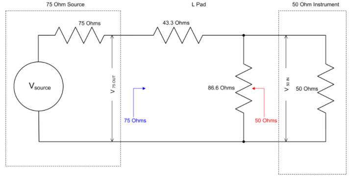
Consider measuring a signal from a 75Ω signal source, such as a camera. The camera’s load is 75Ω. To ensure proper impedance matching between the signal source and the oscilloscope, a 75Ω to 50Ω impedance box is used to match the camera to the oscilloscope and vice versa. An L-type impedance box network is a common MLP. This impedance box connects the input signal with a 75Ω impedance. When looking at the signal source from the output, the impedance is 50Ω. Figure 1 shows the circuit diagram of the MLP for converting 75Ω to 50Ω.
Figure 1: Circuit diagram of the L-type impedance matching box for connecting a 75Ω signal source to the 50Ω input of the oscilloscope.
Through some basic circuit analysis, it is easy to see that when looking at the oscilloscope from the 75Ω source end, the voltage insertion loss of this L-type impedance box is 7.48dB (gain of 0.422). If the oscilloscope is used in default mode, all voltage measurements at the reference MLP’s 50Ω output will be 7.48dB lower. Various built-in tools of the oscilloscope can be used to recalibrate the input measurement and move the measurement plane to the input side of the MLP.
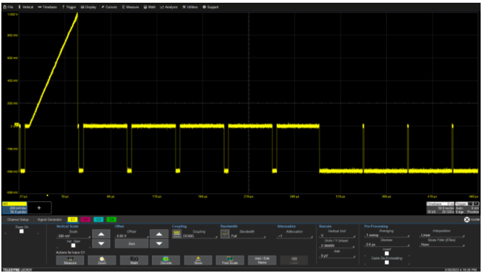
The easiest to use is the input channel recalibration function. The oscilloscope used in the following example has a recalibration function in the channel settings dialog box (Figure 2).
Figure 2: The recalibration function in the channel dialog box allows users to multiply the channel input by a constant or add/subtract a constant and modify the measurement units.
The gain of the above MLP is 0.422. By recalibrating and multiplying the input signal by the inverse of the gain, 2.37, the signal level can be brought back to the full scale value at the MLP input. Measurements are now referenced to the MLP input, and all oscilloscope measurements, including cursor readings and parameters, will read the voltage at that point. The camera now operates at a 75Ω load, while the oscilloscope sees a 50Ω source impedance, and everything is perfect.
The recalibration function can also be used to convert measurement units. This way, readings from sensors or transducers can not only be correctly calibrated but also characterized in appropriate physical units.
Accelerometer Measurement
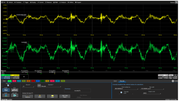
The recalibration function of the oscilloscope mentioned above can also be applied as a mathematical function to input channels or other types of oscilloscope traces. Using mathematical functions allows simultaneous observation of input and output waveforms. Figure 3 shows the basic operation of recalibration, including unit conversion functionality.
Figure 3: The mathematical calibration function provides the same basic operations as channel calibration while allowing users to observe input and output waveforms simultaneously.
The signal source in this example is an accelerometer with a sensitivity of 10mV/g. The accelerometer is mounted on a small air compressor to monitor vertical acceleration. The trace above is the output of the accelerometer, with vertical units in volts. Although the sensitivity of the accelerometer is in mV/g, the industry often simplifies the integration of acceleration into speed and displacement measurements (with units of m/s and m, respectively) using a recalibration constant in mV/m/s². The recalibration function’s calibration method involves multiplying the accelerometer’s voltage signal by the inverse of the sensitivity (units in m/s²/V), specifically 980E-6. Check the ‘Override Units’ checkbox and enter m/s² in the ‘Output Units’ box.
Reviewing the input and output of the recalibration function helps to understand the characteristics of the input, such as offset, overload, and potential clipping issues that may affect recalibration results.
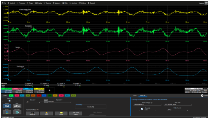
Since the recalibrated measurement unit is now m/s², the acceleration can be integrated into speed and then into displacement, as shown in Figure 4.
Figure 4: The flexibility of recalibrated units allows additional processing of the accelerometer signal using more meaningful measurement units. Each integration operation benefits from adjusting gain and offset, thus eliminating cumulative errors caused by offsets.
The oscilloscope used in this example automatically changes the input unit at each stage of the processing, so after the first integration, the speed trace is seen in m/s. After the second integration, the waveform represents displacement in meters. The peak-to-peak value of displacement is 9.13nm. The fundamental frequency is 53.8Hz, which is related to the induction motor driving the compressor. As observed, the functions of recalibration magnitude and changing measurement units are very useful.
This input channel recalibration function can only be used for its associated channel, while the aforementioned mathematical recalibration function can be applied to various other functions of the oscilloscope. Therefore, if one wants to extend the FFT of a signal from the original dBm value (relative to 1mW) to dB relative to 1V (dBv), it is necessary to subtract 13dB from the dBm reading. When using the mathematical recalibration function at the FFT output, the multiplication constant is kept as 1, while -13 is entered into the constant field, and the unit should be changed to dBv. This completes the recalibration of the FFT, allowing the spectrum to be displayed with vertical units in dBv.
De-embedding Function Example
Cable de-embedding, while related to recalibration, is a more complex process. Recalibration simply multiplies or adds a constant to the waveform, while de-embedding is a process of correcting or removing frequency-related variations in the signal. Basic de-embedding functionality is available in some mid to high bandwidth oscilloscopes. The most basic form of de-embedding is to eliminate the effects of the connecting cable from the measurements. Like recalibration, this will move the measurement plane from the output of the cable to the input.
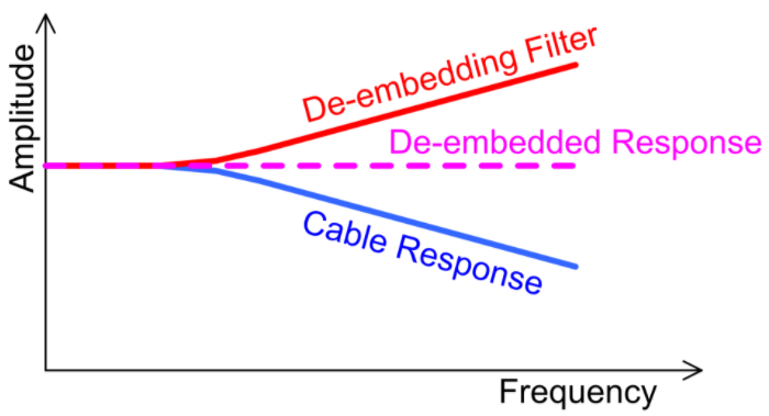
The role of the cable acts like a low-pass filter, limiting the bandwidth of the signal. Like a low-pass filter, it reduces the amplitude of high-frequency signals by filtering out high-frequency components. This also increases the rise time of pulse-like signals. The basic concept of de-embedding is to use a de-embedding filter with a frequency response that is opposite to that of the cable’s frequency response. Generally, cables exhibit a low-pass response, so the de-embedding filter should have a high-pass response. As shown in Figure 5, by combining these, the response will be restored to normal (without the cable).
Figure 5: The basic concept of de-embedding is to utilize a filter with a complementary frequency response to compensate for the cable output signal and counteract the effects of the cable, resulting in a flat frequency spectrum response.
In the user interface of the cable de-embedding function, it is necessary to describe the cable, including its length, propagation speed, and frequency response. The frequency response can be input in tabular form as S-parameters for the forward transfer function (S21) or as the attenuation per 100 feet of cable, which is a function of frequency characterized by constants A1 and A2 in the manufacturer’s frequency response equation. The equation takes the form:
The two terms in the equation represent resistive loss and dielectric loss, respectively.
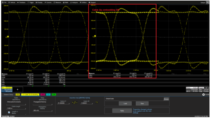
Figure 6 shows an example of cable de-embedding for a 1.25GS/s NRZ waveform connected through a 1-meter RG316 cable.
Figure 6: Cable de-embedding settings for a 1-meter RG316 cable using the above attenuation equation; the inserted part (in red box) shows the signal before de-embedding.
The red box shows the signal before de-embedding. Its average rise time is 236ps, fall time is 236ps, and amplitude (peak-to-peak) is 300.3mV. The de-embedding settings used the above insertion loss equation, with manufacturer-provided constants A1=25.393, A2=3.017, length of 1 meter, and velocity factor of 0.66. After de-embedding, the average rise time decreased by 6ps, the average fall time decreased by 6.4ps, and the average amplitude increased by 10.8mV. Thus, the cable de-embedding function improves the quality of the signal by reducing the effects of the cable.
This cable de-embedding function is standard on this oscilloscope. To perform consistency testing on serial data streams, most high-performance oscilloscopes offer a more complete de-embedding software option, including de-embedding cables, motherboards, and fixtures. These oscilloscopes can perform virtual probing anywhere within the device under test.
Uses of Recalibration and De-embedding
Designers and test engineers should understand that recalibration and de-embedding are very useful functions that can be used to resolve significant measurement errors that may arise from input interface issues.