Improving the accuracy of an oscilloscope is not difficult, but attention to detail is required. This article will explore various methods to enhance oscilloscope measurements.
Using Multiple Grids to Maintain Dynamic Range
A common use of an oscilloscope (4 channels) is to sacrifice one-quarter of its dynamic range by attenuating the amplitudes of several signals so that they can be displayed simultaneously on a shared screen (as shown in Figure 1).
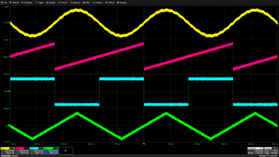
Figure 1: Attenuating the amplitudes of several signals to display them on a shared screen means sacrificing dynamic range.
Generally, digital oscilloscopes are designed to map the full range of their analog-to-digital converter (ADC) to the full or nearly full display grid of the monitor. If the signals from each channel are attenuated to display within one-quarter of the screen grid (two grids), it results in a sacrifice of two digital bits of dynamic range. Furthermore, to display the signal traces within specific grids, a bias must also be added. The bias error introduces another source of error in the readings.
To address the above issues, multiple grid (partitioned) displays should be used, showing each channel signal in separate grids. This way, there is no need to attenuate the signals or apply voltage offsets, allowing multiple channel signals to be displayed with full dynamic range (as shown in Figure 2). In the figure, an orthogonal display shows four partitioned regions with full dynamic range.
When comparing the traces in Figure 1, it is noted that each signal in Figure 2 exhibits lower noise. Utilizing larger vertical scale readings for signal acquisition can reduce the vertical displacement of the input signal but does not decrease the internal noise within the oscilloscope channels.
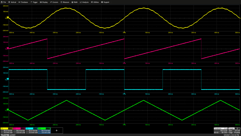
Figure 2: A four-grid (partitioned) display (each channel corresponds to a partitioned display) shows the waveforms of four signals with full dynamic range.
This method results in a lower signal-to-noise ratio, which can be observed by comparing the signal overlay on channel 1 (as shown in Figure 3).
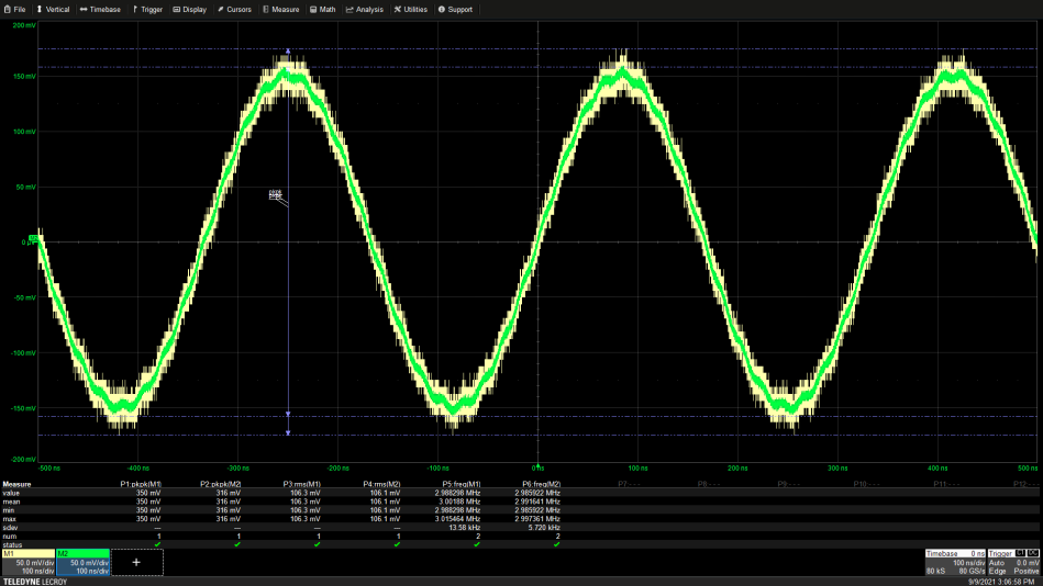
Figure 3: Overlaying the signal acquired at 50mV/div (green trace) with the signal acquired at 200mV/div (yellow trace). The yellow trace is observed to be wider, less defined, and noisier.
When the signal acquired at 200mV/div is attenuated four times and displayed at 50mV/div, it shows greater noise and lower resolution. The unattenuated sine wave trace (green) exhibits smaller disturbances, as the dynamic range has improved.
Display not only shows this amplitude resolution loss but also affects other measurements. Peak-to-peak measurements are very sensitive to noise. Note that the peak-to-peak reading of the attenuated signal has a higher noise level, which is 44mV higher than the result obtained at 50mV/div. However, its root mean square level is very close, as the root mean square process integrates the signal, thereby reducing the measurement’s noise level.
The high noise of the attenuated signal also affects its frequency measurement. It is noted that when expressed in standard deviation, the measurement uncertainty of the attenuated signal is twice as high.
This means that one should not attenuate signals for the sake of using a single grid display—instead, a multi-grid display should be used to show the full dynamic range of each signal.
Accurate Cursor Readings
Oscilloscopes typically provide three measurement tools: screen grids, cursors, and measurement parameters. The cursor is a movable marker on the displayed waveform that can record its position and the waveform amplitude at the intersection with the cursor. The accuracy of cursor measurements depends on the ability to place the cursor precisely at the desired point on the waveform.
Several simple techniques can enhance the accuracy of cursor placement. First, stop signal acquisition when placing the cursor. Each acquired waveform is different, and placing the cursor is much easier when the waveform is stable. Secondly, and more importantly, zoom in on one or multiple traces. Cursor tracking in the zoomed area or a larger display area makes precise cursor placement easier (as shown in Figure 4).
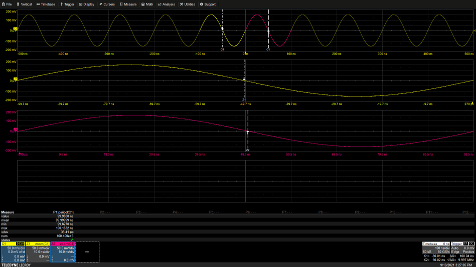
Figure 4: Cursor tracking in the zoomed trace. Using an extended view of the zoomed trace to place the cursor more accurately.
The extended display in the zoomed view not only makes it easier to see waveform details, but also reduces the rate of change when the cursor enters the zoomed area. A slower rate of change allows for better control when placing the cursor.
In the example above, the cursor needs to be placed at the zero-crossing point of the sine wave. Display two zoomed views, each showing one crossing point. Manually move the cursor and monitor the cursor amplitude in the channel annotation box. When the cursor amplitude reading is 0V, the cursor can be set.
Note that the average period of the sine wave measured using measurement parameter P1 is 99.9999ns, while the value measured with the cursor is DX=100.04ns. Measurement parameters provide higher resolution because they use a dual interpolation operation when determining the period. Typically, the measurement results provided by measurement parameters are the most accurate. However, the cursor provides a more convenient measurement tool, as not every measurement has a measurement parameter.
Selective Parameter Measurement
Figure 5 shows a waveform for which it is difficult to establish standard measurement parameters without any assistance. The waveform is the gated clock waveform of the I2C serial interface. The two waveforms in the figure are identical, while the frequency parameter will be used to measure the clock frequency under different measurement configurations.
Parameter P1 measures the frequency of the upper trace. Observing 162 cycles, the measured frequency ranges from 68.518kHz to 100.298kHz. This is not surprising, as the timing of the waveform is not uniform. The reading of P1 is the frequency of the last acquired cycle in the waveform, showing a frequency of 73.281kHz. Looking at the last cycle in the M2 waveform (green trace), it can be seen that it is longer than most of the other cycles, indicating a lower frequency.
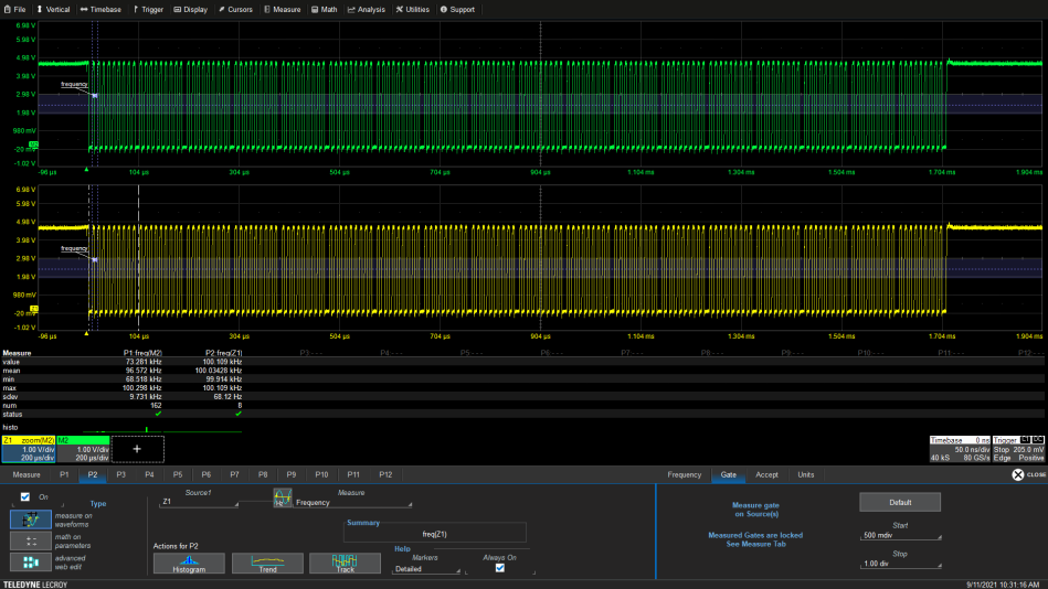
Figure 5: Selectively measuring the gated clock frequency using measurement gates.
Several techniques in parameter settings can be used to address this issue. The first is gating, which, as the name suggests, allows measurements only between gates positioned by the user. Some oscilloscopes use measurement cursors to gate parameter measurements. The Teledyne LeCroy oscilloscope used in this example employs a set of separate gate markers, displayed as dashed lines on the lower (yellow) trace. The gates are set near the first clock and measure the frequency over eight complete cycles. In this case, the frequency parameter readings range from 99.914 to 100.109kHz. The gating successfully limits the measurement to the clock range and ignores the gaps. Gating makes measurement parameters more flexible.
The second measurement tool is the acceptance criterion. This tool allows parameter measurements of all values but only displays values within the user-defined range, as shown in Figure 6:
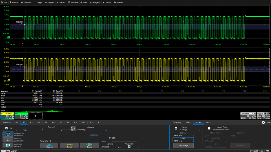
Figure 6: Using parameter acceptance criteria to display frequency values only between 99 and 101kHz.
In parameter P2, the acceptance criterion is set to display only frequencies between 99 and 101kHz. The number of measurements within this range is only 144, while the total count of all measured values listed in P1 is 162. The frequency parameter begins measuring from the first rising edge, so there are 18 gaps in the measured clock waveform, equal to the difference between the total measurements and the accepted values.
Tracking is a mathematical function available in some oscilloscopes that can plot the relationship between parameter values and time. In this case, this function is useful to see which results in the waveform are associated with different waveform events. Figure 7 shows tracking of the frequency parameter.
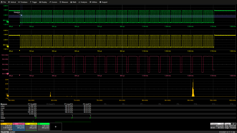
Figure 7: Example of tracking (F2) and histogram (F1) functions based on the measured frequency parameter.
The trace F2 (red) represents the tracking results of the frequency parameter. Its vertical scale is in Hertz, depicting the relationship between frequency units and time. The trace is synchronized in time with the I2C clock source waveform. The maximum value of the shown pulse waveform is 100.3kHz, and the baseline is 68.52kHz. Corresponding to the start and end of the source waveform, each tracking end’s baseline is slightly higher, but the maximum value remains consistent. Tracking can show where frequency changes occur. Note that the 100kHz segment is wider compared to the section below 70kHz, indicating that there are more clock pulses within the 100kHz group.
Trace F1 is the histogram representation of the frequency parameter, displaying the occurrence of measurement data values within a small range relative to the data values. It is an estimate of the probability of measurement occurrences. The histogram for the previously mentioned P1 frequency measurement is shown as trace F1 (yellow) in Figure 7.
The histogram is located at the bottom. The horizontal axis represents measurement values, in this case, frequency. The vertical axis shows the number of measurement values within smaller intervals (bins). The size of the bins can be user-defined. In this case, the horizontal axis is divided into 1000 bins. Thus, for a range of approximately 100kHz, the bin size is about 100Hz. The histogram displays two prominent peaks and two much smaller peaks. The largest peak is at 100kHz, representing a peak count of 34 in the 100kHz bin, with lower counts in the adjacent bins, totaling 144. The leftmost one is at 68.6kHz, which is the clock frequency that includes gaps. The two smaller peaks are also gap frequencies, approximately 72-73kHz, associated with the parameter measurement at either end of the clock signal.
The histogram and tracking results (with most readings around 100kHz) provide the necessary information for selecting and setting acceptance limits in parameter measurements. Values below 100kHz are associated with gaps in the clock burst and should be excluded from the clock frequency measurement.
Tracking and histogram functions provide deeper insights into oscilloscope measurements, showing the original positions of measurement values and how these values are distributed.
Conclusion
This article discussed several techniques to improve oscilloscope measurements, including maximizing display resolution, cursor placement, and measurement parameters. The oscilloscope used in this article is the Teledyne LeCroy Lab Master, which may have similar functions to other oscilloscopes. Tracking and histograms are often associated with jitter measurement tools.