Gaussian processes, also known as normal random processes, are one of the most important and common processes in the field of communications. They represent the main noise in practical communication systems.

The theory presented in this article is primarily derived from “Communication Principles (7th Edition)”. This book provides a substantial mathematical foundation for its concepts, while other texts only briefly touch on them. The MATLAB generation content is sourced from relevant reference books, providing a more intuitive understanding of multidimensional probability density, and it is important to distinguish between various concepts. At the end of the article, a function for generating Gaussian-type random variables (random processes) in MATLAB is provided for reference, and for more details, it is recommended to consult the help documentation.

The content of this article is for my personal learning and understanding, and is for reference only. I welcome any criticism or corrections regarding errors or misunderstandings in the text.

Definition of Gaussian Random Processes

If the joint distribution of any dimension of a random process follows a normal distribution, it is referred to as a normal process or Gaussian process. Its dimensional normal probability density can be expressed as follows:

In the equation, and represent the normalized covariance matrix determinant. It is expressed as:

where

represents the normalized covariance function (two-dimensional probability density function).Note the difference between the variance matrix in the following example and the aforementioned normalized covariance matrix determinant (the matrix corresponding to the determinant). The definitions in the reference books for the following example may differ slightly, but the differences are not significant; however, it is still important to distinguish.

Example of the joint probability density of two-dimensional random variables from “MATLAB-Based Communication System Simulation”. The joint density of two random variables can be displayed through a three-dimensional graph. If its covariance matrix (note that this is the covariance matrix) is given, then its two-dimensional Gaussian distribution is represented as follows:

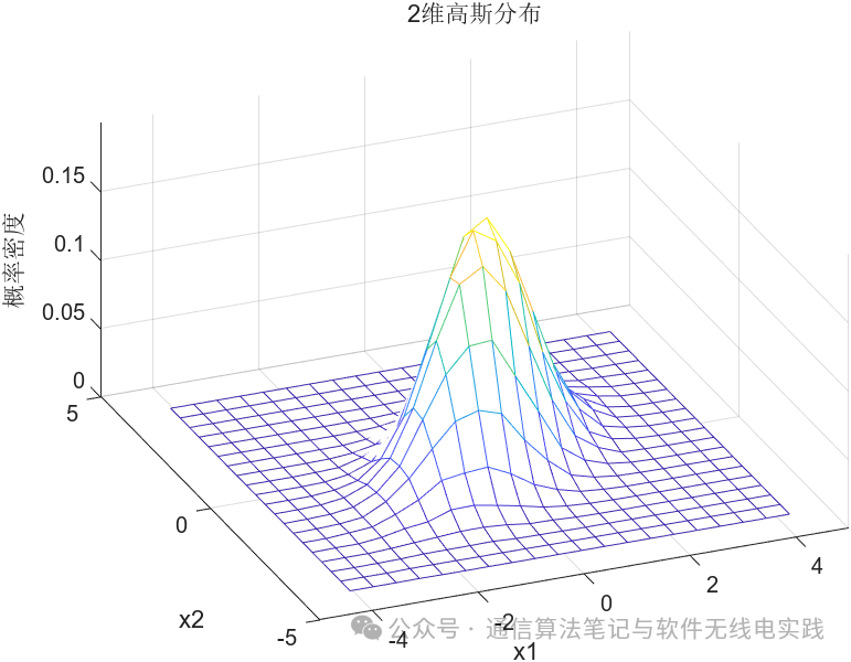
The generation code is found in the aforementioned reference book, but it had errors during execution, which I have modified:

N = 100000; % Sample size
C = [1, 1/2; 1/2, 1]; % Covariance matrix
m = [0, 0]'; % Mean vector
y = zeros(N, 2); % Initialize sample matrix
% Generate Gaussian samples
for j = 1:N
    y(j, :) = gausamp(m, C);
end
% Plot 3D histogram
[N_samp, xx] = hist3(y, [20, 20]); % Use hist3 to generate 2D histogram
x1 = xx{1}; % x-axis boundaries
x2 = xx{2}; % y-axis boundaries
dx1 = diff(x1); % x-axis intervals
dx2 = diff(x2); % y-axis intervals
dx1= dx1(1);
dx2= dx2(1);
% Normalize to obtain probability density
p_hist = N_samp / (N * dx1 * dx2);
% Create grid data for mesh plotting
[X, Y] = meshgrid(x1, x2);
% Plot mesh graph
mesh(X, Y, p_hist);
xlabel('x1');
ylabel('x2');
zlabel('Probability Density');
title('2D Gaussian Distribution');
% Gaussian sample generation function
function y = gausamp(my, Cy)
    % Generate Gaussian process samples
    x = randn(1, length(my)); % Use MATLAB's randn to generate Gaussian random sequence
    y = x * sqrtm(Cy)' + my'; % Generate samples
end

For further understanding, refer to “Communication Principles (7th Edition)”: The above indicates that any dimension follows a normal distribution:

1. When , it means that the random variable at each time point in the random process follows a normal distribution;
2. When , it indicates that the two-dimensional probability density function of any two time points in the random process follows a normal distribution;
3. When , it indicates the three-dimensional or higher-dimensional probability density function.

Important Properties of Gaussian Processes

1. The dimensional distribution of a Gaussian process depends only on the mean, variance, and normalized covariance of the random variables at each time point. Therefore, for Gaussian processes, it suffices to study their numerical characteristics.
2. A generalized stationary (wide-sense stationary) Gaussian process is also strictly stationary;
3. If the values of a Gaussian process at different times are uncorrelated, then its dimensional probability density function can be simplified as: $$f_{n}(x_{1},x_{2}, ext{…},x_{n};t_{1},t_{2}, ext{…},t_{n})=f(x_{1},t)f(x_{2},t), ext{…}f(x_{n},t_{n})$$.
4. A Gaussian process remains a Gaussian process after a linear transformation. In other words, if the input to a linear system is a Gaussian process, then the output of the system is also a Gaussian process. This will be very useful later.

Gaussian Random Variables

The values of a Gaussian process at any time are a random variable that follows a normal distribution (Gaussian random variable), and its one-dimensional probability density function is expressed as:

In the equation, and are the mean and variance of the Gaussian random variable, respectively. It can be represented as shown in the following figure: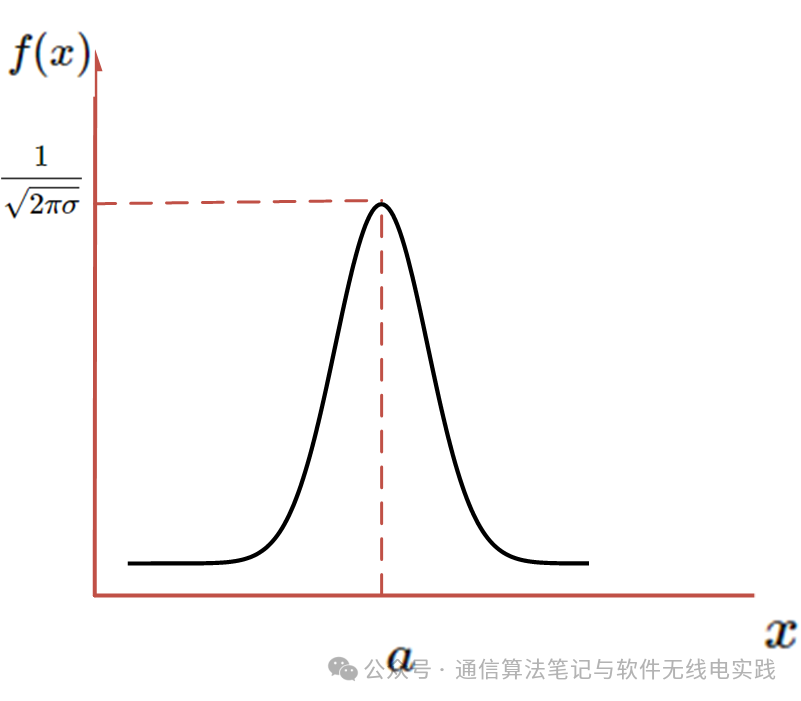

Characteristics of Gaussian Random Variables

1. The probability density function is symmetric about this line;
2. and ;
3. denotes the center of the distribution, denotes the standard deviation, indicating the degree of concentration. The graph becomes taller and narrower as decreases. When is 1, it is referred to as the standard normal distribution.

In performance analysis of communication systems, it is generally necessary to calculate the distribution function of Gaussian-type random variables, which can be expressed as follows:

This integral cannot be computed in closed form, and is generally calculated using some special functions whose values can be found in mathematical handbooks. (Calculation methods)

Error Function, Complementary Error Function, and h-function

Error function and complementary error function representation: For perform a variable substitution, let , then we have , thus:

, in the above equation, denotes the error function. It is defined as:, which is an increasing function of the independent variable, with ; ; . Here, we also introduce a function corresponding to the error function, known as the complementary error function, whoseapproximation formula is:For and its relationship can be derived by oneself;

Another function often used to represent the area under the tail of the Gaussian curve is denoted as , which is defined as:

. With this, the distribution function can be calculated. Its relationship with the complementary error function is:.

In future analyses of communication systems’ noise resistance, the above distribution functions will often be used, and their function values can be calculated through lookup tables or or .When there is no function value table, the function values can be approximated using the complementary error function’s approximation formula.

How to Generate Gaussian-Type Random Variables and Gaussian Random Processes in MATLAB

MATLAB provides the function :

1. Gaussian random variable:;
2. Gaussian-type random process:, generating rows and columns of Gaussian-type random variables, the array composed of Gaussian-type random variables is the Gaussian process.

For specific content, it is recommended to directly consult the MATLAB help documentation: randn

References

“Digital Communication – Fundamentals and Applications (2nd Edition)”

“Communication Principles – Modulation, Coding, and Noise (7th Edition)”

“Communication Principles (7th Edition)”

“MATLAB-Based Communication System Simulation”

randn