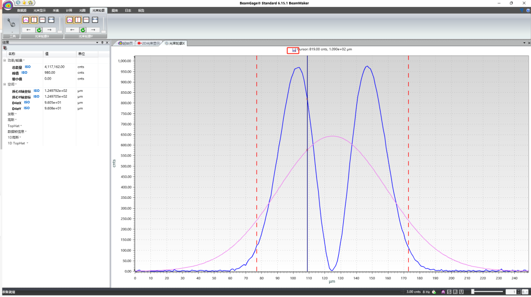
In this issue, we will share how to read data from a CSV file and create plots with a single click. Sometimes, we save data such as spot images or spectra in CSV format, which can be imported into Origin for plotting. However, it can also be easily achieved with just a few lines of code in MATLAB.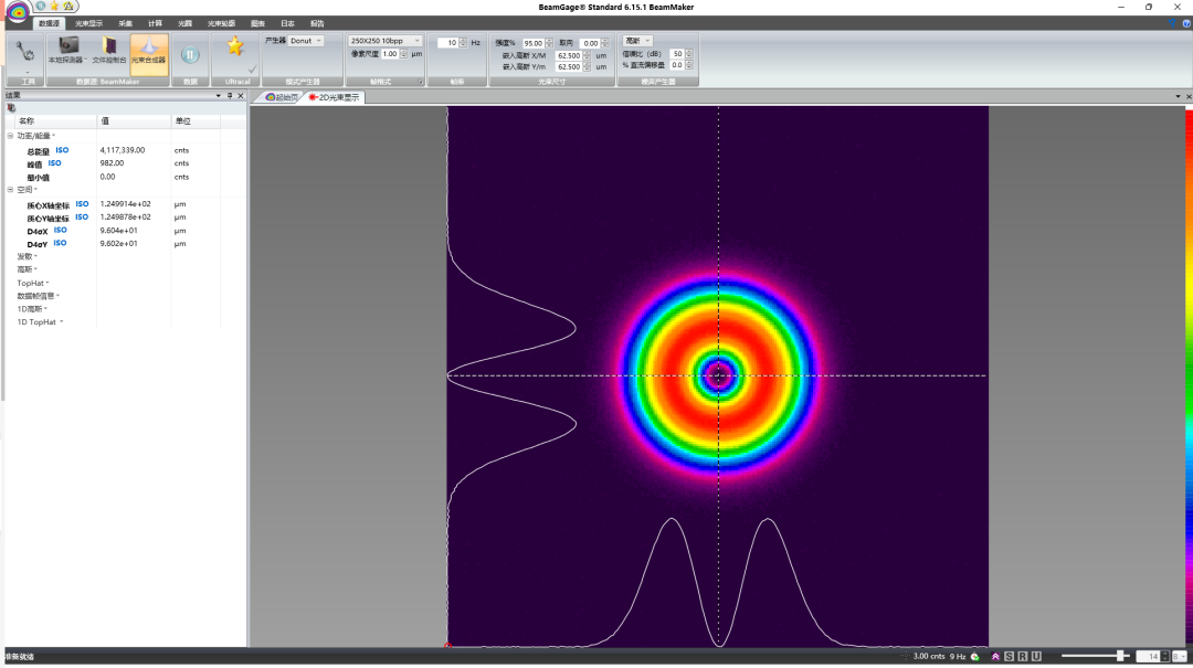 For example, to demonstrate, we simulate the spot of a vortex beam in CCD software to display the beam profile. The data is saved in CSV format.
 First, copy the file path and read the file as a table with headers.
T = readtable("C:\Users\33625\Desktop\test.csv");Next, we proceed with plotting and beautifying the image.
figure('Position',[-1920 0 1920 1200],'Color','w')readdata_to_plot(T,'r','-',2,'$LG}')%% Image beautificationgrid on;box on;xlabel('$\emph{x}\ (\rm{mm})$','Interpreter','latex','Fontname','times new roman','fontsize',20);ylabel('\rm{Normalized\ Intensity}','Interpreter','latex','Fontname','times new roman','fontsize',20);set(gca,'fontname','times new roman','fontsize',20,'BoxStyle','full')legend('show','box','off','interpreter','latex','fontname','times new roman','fontsize',20)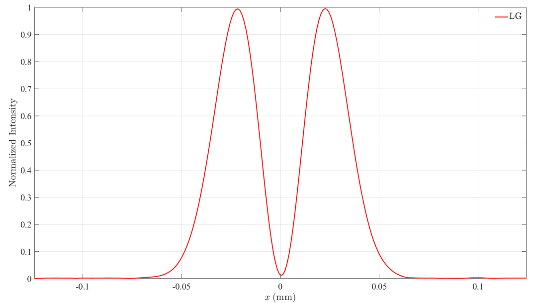 The entire MATLAB program consists of 11 lines. It is important to note that the unit for each element in the software header is 1 micron, which can be adjusted in the function file for the x-axis display. Additionally, the function shifts the entire plot to center by calculating the average value, which is best omitted when plotting spectral data. The function also employs two methods for data smoothing: wavelet denoising and Savitzky-Golay (SG) filtering. This method allows for plotting beam profiles and spectral data from CSV tables.
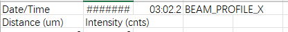 Appendix: Function File
function readdata_to_plot(dataID,linecolor,linestyle,linewidth,legend)%% Read CSV file and plot intensity profile headers = dataID.Properties.VariableNames; % Read file headers % Iterate through each column for i = 1:length(headers) columnName = headers{i}; P{i} = columnName; % Header name columnData{i} = dataID.(columnName);% Convert to data without headers end u1 = columnData{1}; % Read first row of data u2 = columnData{2}; % Read second row of data u2 = u2./max(u2(:)); % Normalize data L = (max(u1)-min(u1))/1000; % Width of x-axis || mm x = linspace(-L/2,L/2,length(u1)); % Generate x-axis xc = sum(x.*u2,'all')./sum(u2,'all');% Calculate beam centroid %% Wavelet denoising [denoised_u2, ~, ~] = wdenoise(u2, 1, 'Wavelet', 'sym4', ... 'DenoisingMethod', 'UniversalThreshold'); %% SG filtering order = 2; frame_len = 21; I_sg = sgolayfilt(u2, order, frame_len); %% Plotting hold on; plot(x-xc,I_sg,'color',linecolor,'LineStyle',linestyle,'LineWidth',linewidth,'DisplayName',legend,'Visible','on'); % Store beam centroid axis([-L/2,L/2,0,1])end