Exploring Advanced Functions of Siemens PLC: PID Control

Introduction: The Charm of PID Control

Hello everyone, I am Ake, a tutorial author fascinated by automation technology. Today we are going to discuss a feature that sounds very “high-end” but is actually very practical— PID control. It plays a role of “stability while seeking progress” in automation control, especially suitable for controlling various “fidgety” physical quantities like temperature, pressure, and flow.

Today’s goal is: to help you understand the core principles of PID control and implement a temperature control case using Siemens PLC. Don’t worry, I will guide you step by step and clarify every detail.

1. What is PID Control? Understand It with Everyday Examples

1.1 What Exactly is PID Control?

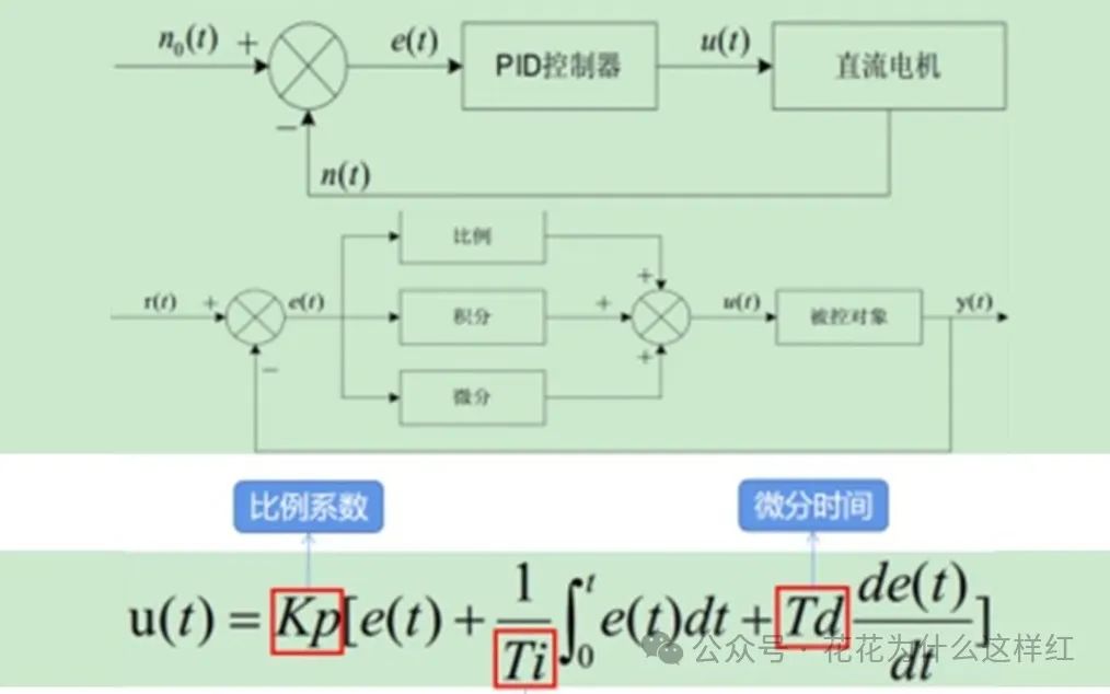
PID control is actually a logical algorithm, named after three core parameters: Proportional (P), Integral (I), and Derivative (D). In simple terms, it is a “smart” controller that keeps your target value (like the desired temperature) consistent with the actual value (like the measured temperature).

P (Proportional): Amplifies the error; the larger the error, the more intense the reaction, similar to slamming the gas pedal while driving.
I (Integral): Accumulates the error to ensure it doesn’t persist over time, like a small map that constantly corrects the direction.
D (Derivative): Predicts the future trend of the error, reacting in advance, like an experienced driver’s anticipation.

1.2 An Everyday Example

Suppose you are boiling a pot of soup, and the target temperature is 80°C.

When the soup’s temperature is only 40°C, you would turn the heat up to maximum (Proportional Control).
As the temperature approaches 80°C, you would gradually reduce the heat to prevent exceeding the target value (Derivative Control).
If you find the temperature hovering around 78°C, you might slightly increase the heat to stabilize it at 80°C (Integral Control).

This is the basic idea of PID control.

2. PID Function in Siemens PLC

2.1 PID Modules in Siemens PLC

The Siemens S7-1200 and S7-1500 series PLCs come with powerful PID function blocks, such as PID_Compact and PID_3Step. These function blocks allow us to easily implement PID control without having to write complex algorithms ourselves.

Inputs and Outputs of Function Blocks

Inputs:

* **Setpoint**: Target value, such as 80°C.
* **Process Value**: Actual measured value, such as the current temperature of 70°C.
* **Mode**: Choose between automatic control or manual control.

Outputs:

* **Control Variable**: For example, the power output to the heater, ranging from 0% to 100%.

Advanced Features of PID Function Blocks

In addition to the basic PID algorithm, Siemens’ function blocks also provide many “user-friendly” features, such as:

Anti-Integral Saturation: Prevents excessive control output that could lead to system instability.
Output Limiting: Restricts the maximum and minimum output values to avoid damaging equipment.
Self-Tuning Function: Automatically calculates appropriate PID parameters, eliminating tedious debugging processes.

2.2 Manual/Automatic Switching of PID

In industrial settings, it is often necessary to switch between automatic and manual control. For example:

Automatic mode: The PID function block controls the output based on the algorithm.
Manual mode: The operator directly adjusts the output value.

The PID function block in Siemens PLC supports smooth switching, such as:

When switching from automatic to manual, the current output value is directly passed to manual mode.
When switching from manual to automatic, the current process value is taken as the setpoint to avoid sharp fluctuations in the system.

3. Hardware Wiring and Ladder Diagram Implementation

3.1 Hardware Wiring

Example: Temperature Control System

Assuming we want to control the temperature of a heating furnace, the required hardware includes:

Temperature Sensor (such as thermocouples or PT100): Connect to the PLC’s analog input module.
Heater (such as a solid-state relay-driven heating rod): Connect to the PLC’s analog output module.

The wiring diagram is as follows:

+-----------------------------------+
| Temperature Sensor -> PLC Analog Input (AI0)  |
| PLC Analog Output (AQ0) -> Heater       |
+-----------------------------------+

3.2 Ladder Diagram Program

In the ladder diagram, we use Siemens’ PID_Compact function block. The program logic is as follows:

Input Setpoint: Target temperature.
Input Process Value: Measured value from the temperature sensor.
Output Control Variable: Power of the heater.

Here is a simple example of a ladder diagram:

+-----------------------------------------------+
| PID_Compact Function Block                             |
| Input: Setpoint (target temperature), Process Value (measured temperature)  |
| Output: Control Variable (heater power)                     |
+-----------------------------------------------+

4. Code Example: Implementation of PID_Compact

4.1 Parameter Configuration

In Siemens’ TIA Portal, after dragging in the PID_Compact function block, configure the following parameters:

Setpoint (Target Temperature): For example, set to 80°C.
Process Value (Sensor Input): Connect to the analog input module.
PID Parameters:

* Proportional Gain: 0.5
* Integral Time: 10 seconds
* Derivative Time: 1 second

4.2 Program Code (Pseudocode Example)

// Input process value (temperature sensor signal)
Input Process Value = AI0 Signal
// Set target temperature
Target Temperature = 80.0°C
// Call PID_Compact function block
PID_Compact(
    Target Temperature,
    Input Process Value,
    Output Control Variable
)
// Output to heater
AQ0 = Output Control Variable

5. Practical Application Case: Temperature Control of Heat Treatment Furnace

Suppose we need to control the temperature of an industrial heat treatment furnace, aiming to maintain the temperature at 80°C.

Step 1: Connect the Sensor and Heater

The temperature sensor connects to the analog input terminal AI0.

* The heater connects to the analog output terminal AQ0.

Step 2: Use the PID Function Block

Set the target temperature to 80°C.

* Enable the PID function block for automatic control.

Step 3: Debugging and Optimization

Activate the self-tuning function to let the PLC automatically calculate the best PID parameters.

* If the control effect is not ideal, manually adjust the proportional, integral, and derivative parameters.

6. Common Questions and Solutions

6.1 Why is there no response from the output?

Check if the process value input is correct: Use a multimeter to measure the sensor signal and ensure the wiring is correct.
Check the PID parameters: If the proportional gain is too low, the output may respond slowly.

6.2 What if the output fluctuates too much?

Adjust the derivative time: Properly increase the derivative time to reduce system overshoot.
Enable the anti-integral saturation function: Prevent excessive accumulation of the integral term that could cause system oscillation.

7. Precautions

Ensure voltage level matching during wiring: The voltage range of the analog inputs and outputs must be consistent with the equipment.
During debugging, start with low-power loads: Prevent program logic errors from damaging equipment.
Avoid live operations: Always cut power before wiring to ensure safety.

Conclusion: Start with Small Projects and Gradually Master PID Control

Beginners can start with simple temperature or level control projects to gradually familiarize themselves with the principles and parameter adjustment methods of PID control. Later, they can try more complex process controls, such as multi-section temperature control or pressure compensation.

Although PID control sounds complex, with patient practice, you will definitely master it and become a “master” in the field of automation control!

Like and Share