Note:“Development of Fault Injection Methods and Fault Coverage Analysis for Safety-Critical SoCs” is a series of articles consisting of two parts: “Part 1” and “Part 2”.
This is “Part 2”, where we will detail the FIeVC itself and the preparatory phase scripts in Section 2. Section 3 explains the steps to execute a complete fault simulation activity through XFS for comparison with commercial fault simulation tools. Section 4 presents the results obtained using FIeVC and compares them with those obtained through XFS. Finally, the series concludes with Section 5, which discusses future implementations and ideas, and provides concluding remarks.
The “Part 1” of this series has been published and can be accessed here: Development of Fault Injection Methods and Fault Coverage Analysis for Safety-Critical SoCs (Part 1)
Original authors: Alfredo PAOLINO, Matteo SONZA REORDA, Mariagrazia GRAZIANO, Carlo RICCIARDI, Maria Silvia RATTO, Alberto RANERI
Translation: Yuan Dongdong, Yuan Xixi


02. Fault Injection and Verification Component (FIeVC)
A fault simulator is a software tool used to compute the behavior of a circuit in the presence of faults, helping users develop robust diagnostic tests and verify whether safety mechanisms meet fault injection testing requirements.
Fault simulation can be executed using different algorithms. FIeVC is based on a parallel algorithm that strikes a good balance between the low complexity of serial algorithms and the high performance of concurrent algorithms. More complex techniques (such as deductive and differential methods) are not considered to avoid getting bogged down in their theoretical details.
The main advantages of FIeVC include:
・Non-intrusive environment: Despite being built on top of an existing verification environment, FIeVC is completely transparent to it. In fact, it only acts on the DUT without touching the underlying verification environment.
・Ease of use: By simply defining or not defining the environment variable BST_FAULT_SIM, users can switch between the fault simulation process and the functional verification process. With the help of ifdef directives, it can be checked whether this variable is defined and compile the test platform and required files accordingly.
・Adaptability: FIeVC can handle designs ranging from basic to very complex levels. Due to the extensive use of regular expressions and BST naming conventions, the files that make up FIeVC automatically adapt to the current DUT before the compilation stage, requiring no extra effort from the user.
・Flexibility: FIeVC can be easily extended or modified. Since task isolation is done in different files, for example, the analysis can be extended to new fault models by simply modifying one file.
2.1 General Parallel Fault Simulator Structure
For simplicity, FIeVC only parallel simulates two circuits: the golden circuit and the faulty circuit. However, by making slight modifications to the preparatory scripts (Section 2.2) and the environment itself (Section 2.3), the degree of parallelism can be increased, thereby enhancing performance.
The overall structure of the parallel fault simulator is shown in Figure 2.1. The green part represents the original BST verification process, while the red part represents the additional components required for fault simulation.
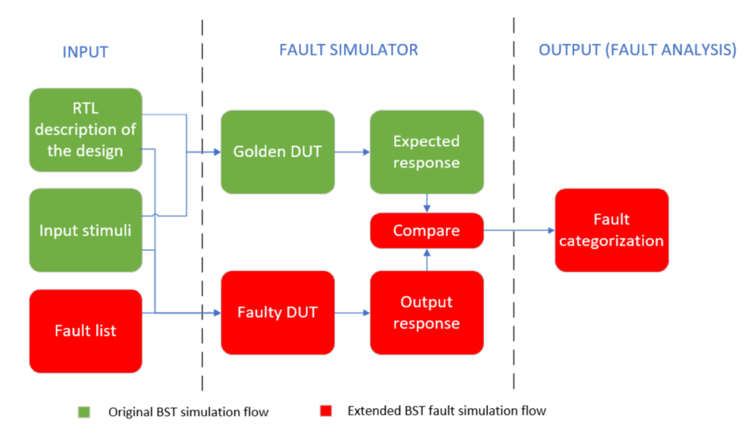
Figure 2.1. Parallel Fault Simulator Diagram
The additional elements required to execute fault simulation include:
・Fault List: A file containing all the injective faults in the design.
・Additional DUT: To ensure accurate reference results, a fault-free golden simulation must run in parallel with the faulty simulation, meaning a single DUT is insufficient, and the test platform must be re-adapted for this purpose.
・Auxiliary Signals: These signals simplify the comparison process, allowing output comparisons to be performed directly within the test platform. The main advantage of this solution is that it allows FIeVC to operate without needing to know the specific details of the DUT, thus greatly enhancing its generality and flexibility. Section 2.2.2 will detail these signals.
・Fault Injection and Analysis Tools: This is the core task of FIeVC.
2.2 Preparatory Scripts
As mentioned in Section 2.1, some preparatory operations need to be performed before fault simulation can take place. However, manually implementing these functions is cumbersome and severely impacts the tool’s flexibility and ease of use. Therefore, the generation of the fault list and the re-adaptation of the test platform are entirely handled by two scripts: a Tool Command Language (TCL) script for generating the fault list and a Python script for re-adapting the test platform.
2.2.1 Fault List Generation Script
The goal of this script is to generate a text file where each line contains a fault.
A typical fault item is characterized by three parameters: fault point, fault type, and injection time (Section 2.3.1). However, this script only outputs a list of injective fault points rather than complete fault items. This way, the fault type and injection time can be managed directly by FIeVC; whenever a fault point is selected from the list, FIeVC will determine the specific fault to inject (such as SA0, SA1, etc.) and the time based on the settings defined by the user in the sequencer (Section 2.3.5) and BFM (Section 2.3.6).
The choice of TCL over Python for this script is due to its ability to be executed as a pre-simulation script through the TCL command line interface (CLI) of the XceliumTM simulator. This setup allows for the automatic retrieval of all input ports, output ports, and internal networks of the design while accessing the compiled design (using the find command).
The steps executed by this script are as follows:
・ Ask the user for the injection range, supporting multiple components and recursive injection.
・ Execute the TCL find command on these components to retrieve input ports, output ports, and internal signals.
・ Split vector signals into single-bit signals to make them injectable.
・ Change the signal path from :dut:* to :dut_faulty:* to ensure faults are injected into the faulty DUT (not the golden DUT).
・ List all obtained fault points line by line in a text file.
2.2.2 Test Platform (TB) Re-adaptation Script
This script is responsible for all tasks related to re-adapting the test platform to create an environment that supports fault injection and analysis. The goal is to replicate the DUT for fault injection and add comparison logic for fault analysis.
Since this script directly modifies the test platform and FIeVC files, it must be executed before the compilation stage to ensure that the environment used during simulation is up to date.
Regarding the first task (DUT replication), a complete parsing of the DUT instantiation in the VHDL design and test platform is required to retrieve all the information needed for replication (input/output signals, generic/port mappings, and signal assignments). With this data, the script can declare a second DUT, changing its name from “dut” to “dut_faulty” and renaming all outputs from “*” to “*_faulty”. The reason for renaming is simple: having two components with the same output signals would generate multi-driven network errors. Finally, the input names are also changed from “*” to “*_buf”, the reason for which will be explained in detail in Section 2.6.1.
Regarding the second task (implementation of comparison logic), there are two options:
・ Introduce the outputs of the DUT and faulty DUT into FIeVC and implement the comparison logic therein.
・ Implement the comparison logic directly within the test platform.
The first method may be more conventional as it ensures that FIeVC is the only component handling the fault simulation process. However, it comes at a high cost: the unknown number of outputs means that comparing all golden outputs and faulty outputs requires a loop that compares them one by one in each clock cycle, which significantly impacts the total simulation time.
The second method moves part of the fault simulation process outside of FIeVC but guarantees greater flexibility, and since the test platform is already being restructured, the cost is zero. Therefore, this method was chosen.
However, before explaining the comparison logic, it is crucial to briefly describe the structure of the fault-tolerant module. As shown in Figure 2.2, these modules consist of a functional module and a safety mechanism connected to it. The functional module is the functional part of the design that implements the required functionality; the safety mechanism is the safety part that checks for possible errors within the module. Therefore, the outputs of the fault-tolerant module are also divided into functional outputs and safety outputs.
Fortunately, in the BST design, the safety outputs can be distinguished from the functional outputs by the string “_fail” at the end of the signal name.
Based on this, the new signals required for the comparison and analysis process include:
・ Each output corresponds to a “*_xor” signal. These signals take the XOR value of “*” and “*_faulty” to indicate where errors propagate.
・ “mismatch_detected” signal: performs an OR operation on all the above “*_xor” signals, meaning that when at least one functional output has a mismatch, this signal is set to ‘1’ (Figure 2.3). Before performing the OR operation with other signals, the vector “*_xor” signals must be compressed to a single bit.
・ “fail_detected” signal: similar to “mismatch_detected” but for safety outputs (Figure 2.4). This signal notifies the safety mechanism that an error has been detected, triggering the fault analysis process.
Finally, the last operation performed by the script is to populate the FIeVC signal mapping (Section 2.3.2) to allow direct access to all these signals from FIeVC.
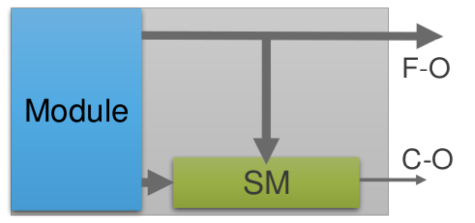
Figure 2.2. Functional Unit Representation
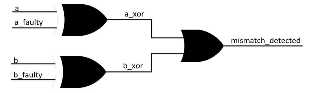
Figure 2.3. Simplified Representation of “Mismatch Detected” Logic
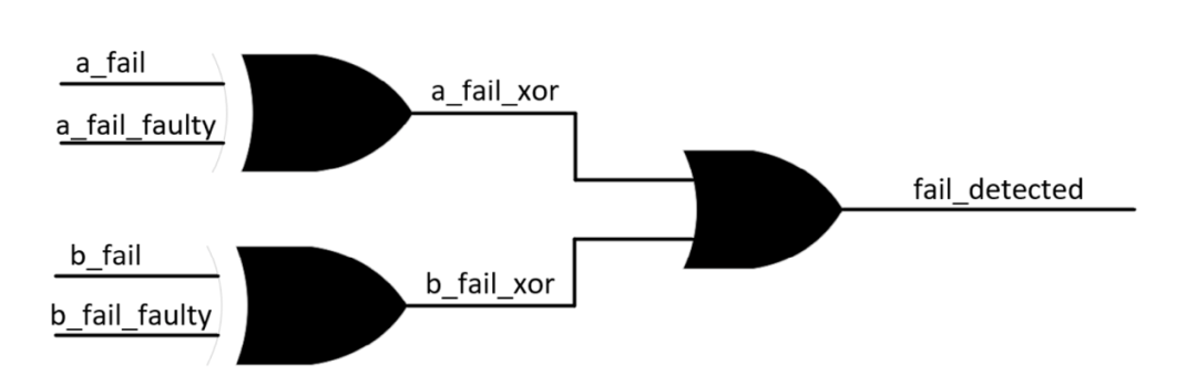
Figure 2.4. Simplified Representation of “Fault Detected” Logic
2.3 FIeVC Structure
With the setup required for fault simulation ready, let’s now look at how fault injection and analysis are implemented.
Correctly implementing these two concepts is key to successfully conducting fault simulations and is the core issue addressed by this paper—FIeVC.
Figure 2.5 shows the structure of FIeVC and how it connects to the test platform. The upper half of the figure represents the modified test platform, while the lower half shows the internal components of FIeVC: signal mapping, monitor, analyzer, sequencer, and BFM. All these components are declared in a component called “Env”, which acts as a wrapper and binds the input ports to the output ports to establish the required connections.
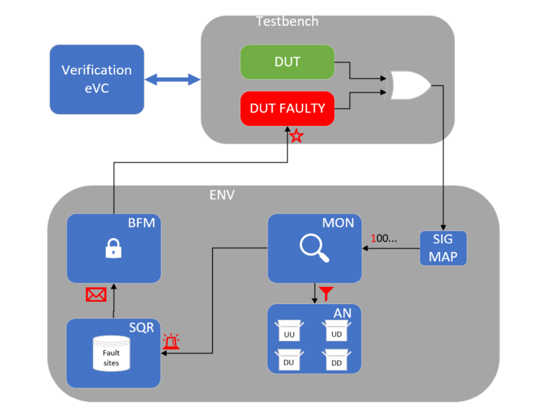
Figure 2.5. FIeVC Structure with Simplified Connections
The connections between the above components are implemented through “e ports” in Specman e, which are equivalent to the more commonly known transaction-level modeling (TLM) ports. The e ports enhance portability and interoperability by separating FIeVC from the DUT.
There are two ways to use e ports:
・External Ports: Create connections between the simulation object (everything within the test platform) and the FIeVC components.
・Internal Ports (e2e): Create connections between two FIeVC components.
In terms of port types, two main types are primarily used:
・Simple Ports: Used for direct access and data transfer.
・Event Ports: Used to transmit events between units to trigger or synchronize.
The following sections will explain all FIeVC subcomponents in detail.
2.3.1 Fault Items
To facilitate the transmission of information about the currently injected fault and the next fault, it is necessary to define an atomic description of the fault that can be accepted by the e port.
Therefore, the term “fault item” is used to model physical faults. A fault item consists of three parameters:
Fault Point: Indicates the network where the fault should be injected. The fault point is randomly extracted from the fault point list by the sequencer (Section 2.3.5) and assigned to the fault item.
Fault Type: Indicates the category of the fault model to be injected (e.g., SA0, SA1, SEU, etc.). The fault type is also randomly selected from the user-declared fault types by the sequencer (Section 2.3.5) and assigned to the fault item.
Injection Time: The time at which the error should appear and manifest in the circuit. Since the current version of FIeVC only considers SAF, the injection time is automatically set to a moment between the end of reset and the start of the test run.
2.3.2 Signal Mapping
This component is automatically generated by the test platform re-adaptation script (Section 2.2.2) based on the auxiliary signals included in the test platform, acting as a connector between the test platform and FIeVC, allowing direct access to all “*_xor”, “mismatch_detected”, and “fail_detected” signals through simple ports. By binding the simple ports to the full HDL path of the required signals, this component continuously reflects the value of the signals, making them accessible from FIeVC.
2.3.3 Monitor
The monitor is responsible for tracking all changes in the comparison logic signals to detect possible mismatches and execute necessary operations. This component performs the following three functions:
・ generate_fault(): Whenever a new injection can be executed, the monitor notifies the sequencer through an event port called “generate_next_fault”.
・ monitor(): The simulation of the currently injected fault continues until the end of the test or until a mismatch is detected in the safety output through the “fail_detected” signal. When either of these two situations occurs, fault classification can be performed in the analyzer (Section 2.3.4) and the next injection can be prepared.
While executing this function, the monitor waits for either of these two events to trigger the analysis and advance to the next injection. At the same time, it checks whether the “mismatch_detected” signal indicates a mismatch, as the analyzer needs this information to classify the fault correctly.
・ update_tlm_ports(): The simulation times of the first mismatch and the first fault occurrence are also saved and passed to the analyzer for classification through TLM analysis ports called “mismatch_time_port” and “fail_time_port”. These ports are similar to e ports but support multiple connections and broadcasting.
2.3.4 Analyzer
Whenever the simulation of a fault item ends (due to fault detection or test completion), it can be classified based on the results obtained.
For ease of subsequent comparisons, the analyzer implements the same fault classification as XFS (Figure 2.6).
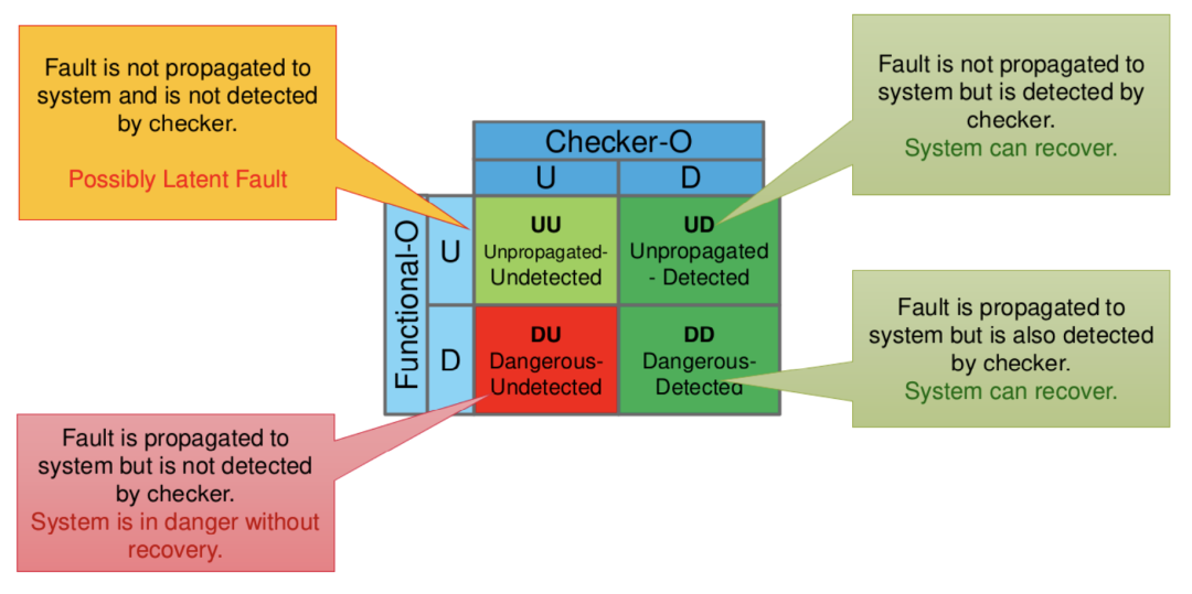
Figure 2.6. FIeVC Fault Classification
Faults are thus classified into four categories:
・Unpropagated Undetected (UU): The fault is neither propagated to the functional output nor detected by the safety output. In this case, no definitive conclusion can be drawn, but the fault may potentially be a safety fault.
・Unpropagated Detected (UD): The fault is not propagated to the functional output but is detected by the safety output. In this case, the system can recover.
・Danger Undetected (DU): The fault propagates to the functional output but is not detected by the safety output. In this case, the system is in a dangerous state as it cannot recover from this error.
・Danger Detected (DD): The fault is propagated to the functional output and detected by the safety output. In this case, the system can also recover.
This component performs the following three functions:
・ init_report(): The first step in conducting a comprehensive analysis is to generate a report file to save all injected results.
The file contains four fields: fault point, fault type, fault category, and FRTI. This function creates a new file and initializes it with these four fields.
・ analyze_fault(): After the analysis is triggered, the values of “mismatch_time” and “fail_time” are read from the two TLM analysis ports. With these two time values, it can be checked whether and when the fault propagated to the functional output or safety output and classify it (Figure 2.7). Saving the difference between “fail_time” and “mismatch_time” (FRTI) allows the user to check whether any safety mechanisms violated their timing constraints.
・ generate_summary(): After the fault simulation activity ends, the total counts of UU, UD, DU, and DD are written to the end of the report file.
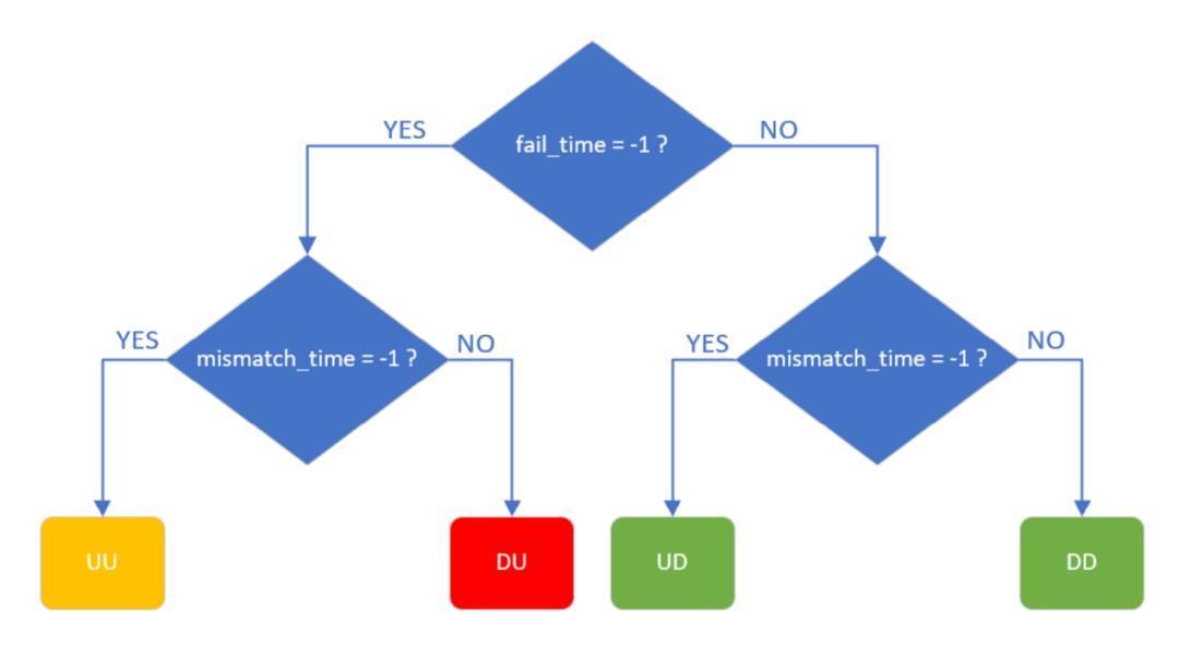
Figure 2.7. FIeVC Fault Classification Process
2.3.5 Sequencer
The sequencer acts as a fault item generator, connecting to the monitor through the “generate_next_fault” port, receiving notifications whenever a new fault item is needed. Unless the user stops it, the fault simulation will continue until all possible faults are injected. At this point, another event port “fault_list_over” is used to trigger the end of the simulation phase.
This component performs the following two functions:
・ fill_fault_sites_list(): At the start of the simulation, the sequencer reads the fault point list generated by the fault list generation script (Section 2.2.1) and creates some internal copies using string lists (one list for each fault type). Although creating these copies slows down the startup process, it saves a significant amount of time in the long run. The main advantage is that whenever a new fault item needs to be created, there is no need to access and re-read the file, thus reducing file access times and shortening simulation time.
・ pick_fault(): After the previous function completes the setup, the process of creating a fault item mainly involves selecting a fault point from the list and assigning the corresponding fault type and injection time. This function is triggered by the “generate_next_fault” port.
2.3.6 Bus Functional Model (BFM)
BFM acts as the fault injector for the system, hence also referred to as the “driver”.
This component performs the following two functions:
・ force_fault: At the start of the simulation and after the analysis phase of the injected fault, the BFM retrieves new faults from the sequencer and injects them into the DUT by executing the command “force (fault_item.fault_site) (fault_item.fault_kind)” on the simulator.
・ release_fault: Before allowing a new injection cycle to begin, the BFM must release the old fault by executing the command “release (fault_item.fault_site)” on the simulator.
2.4 Simulation Process
By assigning different tasks to these components, the simulation process becomes very linear and manageable, divided into three phases: initialization phase, core phase, and ending phase. In each phase, the components perform one or more functions. It is worth noting that the complexity of all functions is completely hidden from the user, who only needs to start the simulation using the xrun command with the desired flags. The complete simulation process is illustrated in Figure 2.8.
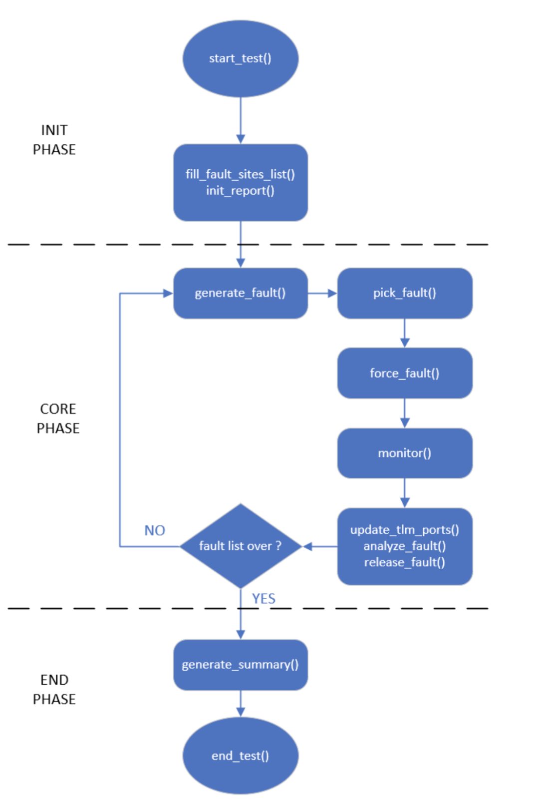
Figure 2.8. FIeVC Fault Simulation Process
2.5 Using Testflow Function to Reset DUT
So far, the described process has not considered a simple but critical limitation: whenever the BFM performs a new injection, the DUT needs to be reset and the test must be rerun from the beginning.
Resetting the DUT is necessary because the previous error may have propagated through the circuit and damaged timing elements, thus the DUT must be restored to a known safe state. The first solution that comes to mind is simple: close the simulation and restart it, injecting the new fault at the start of the new simulation.
Although it sounds easy to solve, implementing this solution incurs a high overhead in simulation time, primarily because the XceliumTM simulator takes time to open and retrieve design snapshots. Additionally, the fault list generated in the sequencer will become useless as they will be overwritten every time the simulation is restarted, making it impossible to track the injected faults. This means that it is necessary to roll back to the single fault list contained in the file, further increasing simulation time. Considering all the drawbacks of this solution, we took the time to explore all the tools and features provided by Specman e to see if a more efficient solution could be implemented.
The solution found relies on advanced Testflow features, significantly enhancing the performance of FIeVC.
By making the FIeVC components and the tests themselves “Testflow-aware”, the simulation and test execution can be divided into multiple sub-phases. With this structure, the simulator ensures that a unit only enters the next phase after all activities in the current phase are completed. Thus, the simulation shifts from a single-threaded execution of the test to a multi-threaded version.
There are eight predefined phases, of which FIeVC uses six, including:
・ENV_SETUP: Initiates the dispute to start the test.
・RESET: Resets both DUTs to accept new injections.
・INIT_DUT: Initializes the faulty DUT with the newly injected faults after reset but before test execution.
・MAIN_TEST: Starts the test sequence after the faulty DUT is ready.
・FINISH_TEST: Pauses the test sequence when the test sequence ends or a mismatch in safety output is detected. From here, fault analysis begins, and the test returns to the restart phase.
・POST_TEST: After processing the fault list, the test does not return to the reset phase but continues to dispute resolution and ends naturally.
The main advantage of this method is that it allows the test to be restarted from a specific phase at runtime, regardless of which phase is currently being executed.
By leveraging these phases, built-in synchronization features, and re-running capabilities, it is possible to repeatedly reset the DUT whenever a new injection is needed.
As shown in Table 2.1, the functions mentioned in Section 2.3 are now transformed into threads, with each thread executing in a specific Testflow phase.
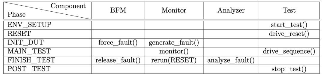
Table 2.1. Thread Allocation for Different Testflow Phases
2.5.1 Simulation Process Using Testflow Features
The process with this new feature is very similar to the one described in Section 2.4, but it focuses more on the execution of Testflow phases rather than individual functions, as shown in Figure 2.9.

Figure 2.9. FIeVC Fault Simulation Process with Testflow Features Enabled
2.6 Backward Propagation Issues
Unfortunately, during initial testing on the SMI240, an abnormal behavior was observed when injecting certain faults. Specifically, some faults seemed to appear on safety outputs that do not belong to the forward cone of the injected node logic. The golden DUT also detected the fault effects, leading to a complete simulation failure, indicating a problem in the environment. To make FIeVC usable, it is essential to understand the root cause of this issue and resolve it. By manually checking signal propagation on the schematic tracker, the cause of this behavior was identified. The circuit response after injection is shown in Figure 2.10. From the figure, it can be seen that forcing a signal value simultaneously forces all connected signals to take the same value, regardless of whether they belong to forward or backward cone logic.
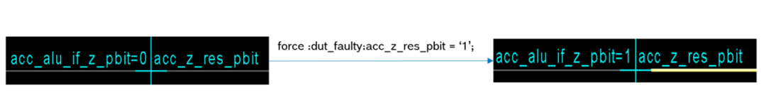
Figure 2.10. Force Command Propagation Error
Therefore, the problem arises from the lack of protection against backward propagation of injected faults in the force command of the XceliumTM simulator, causing faults to propagate throughout the network until the driving end. This means that the injected signal is always equivalent to injecting its driving end and the entire network.
Considering that no elements are inserted between the VHDL port mapping of the two signals, it is likely that there exists a large network composed of different signals in the design. Depending on the position of the driving end, backward propagation is divided into external backward propagation and internal backward propagation, both of which require countermeasures to prevent propagation.
2.6.1 External Backward Propagation
In both types of backward propagation, external backward propagation directly leads to the inability to perform fault simulation, so a solution must be found.
This type of backward propagation is observed when the injected node is directly connected to the input of the faulty DUT. This means that the driving end of this node is located outside the faulty DUT while driving both the faulty DUT and the golden DUT. This structure, combined with the aforementioned behavior of the force command, leads to faults propagating from the faulty DUT to the golden DUT, as the injection occurs at the output of the external driving end.
The solution to this problem is to insert buffers between all input lines of the faulty DUT and their corresponding original driving ends (Figure 2.11), making the driving end of the input signal the buffer itself, thus narrowing the injection range to only the faulty DUT. The buffer insertion is implemented through the test platform re-adaptation script, as described in Section 2.2.2.
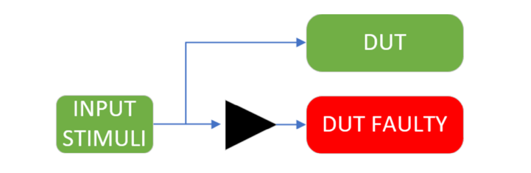
Figure 2.11. Extended Test Platform Structure to Address External Backward Propagation Issues
2.6.2 Internal Backward Propagation
Unfortunately, for the same reasons, this issue arises not only at the boundaries of the faulty DUT but also within the components themselves. This means that faults cannot be injected on the inputs of components/gates, only on the outputs (since the outputs are the driving ends of the entire network). This is undoubtedly a limitation of FIeVC that must be considered when performing fault simulations.
To temporarily address this issue, the fault list generation script (Section 2.2.1) was modified so that the generated list does not contain the signals themselves but their driving ends. Before simulation, the generated driving end list is reprocessed to remove duplicates. This solution allows for the completion of the entire fault simulation and comparison with XFS results, with the downside being that the fault injection range is narrowed down to only partially injectable nodes.
Here are two potential solutions that were not implemented in the final version of the paper:
・ Use the fast recompile feature of the Xcelium™ simulator for dynamic buffer insertion: Fast recompile allows for the recompilation of a single VHDL file in the entire design, reducing the time required for subsequent compilations. In this way, buffers can be added where needed, recompiling the file and executing the simulation. However, this solution is incompatible with Testflow features, leading to a significant drop in performance.
・ Create a new Python script that duplicates each file in the design and adds buffers to all components.
03. Xcelium Fault Simulator (XFS)
3.1 Main Features
XFS is an easy-to-set-up fast tool that runs within the existing XceliumTM simulator compilation engine, allowing seamless reuse of functional verification environments. This means that a complete fault simulation activity can be set up and executed simply by extending the simulation process, without any modifications to the pre-existing environment.
In contrast to FIeVC, XFS only supports serial fault simulation algorithms when handling VHDL components. Additionally, the tool lacks the fast reset feature provided by FIeVC through Testflow functionality, meaning that the only way to perform multiple injections in sequence is to close the running simulation, restore the compiled snapshot, and restart the simulation from scratch. Section 4.1 will demonstrate how the absence of these two features impacts overall performance.
In addition to all files belonging to the original verification environment, using XFS also requires two new files:
・Fault Specification File: This file passes preliminary information about the fault simulation to XFS. Specifically, it uses the command fault_target, followed by the path of the component or subcomponent where the fault injection will occur. This command also accepts two flags: -type to specify the type of fault to inject (SA0, SA1, SET, SEU, or all), and -select to specify the type of network to inject (only ports, cells, or timing signals).
・Gate File: This file is used to define the division between functional outputs and checker outputs, as described in Section 2.2.2. To enhance the reusability of this process, the tool uses another TCL script to automatically set functional outputs and checker outputs by analyzing the output ports of the components during the compilation stage. Finally, this script is also used to specify the gating events of the signals. When simulating the faulty DUT and triggering these events, the current values of all signals will be compared with the expected values.
3.2 Simulation Process
The overall simulation process differs significantly from the one used by FIeVC, especially due to the different algorithms employed.
Using a serial algorithm means that only one DUT can be simulated at a time, so the golden simulation of the fault-free DUT must be performed first. This simulation is executed using the classic xrun command. By using the gating events defined in the gate file, the expected behavior of the golden DUT is extracted and saved to a so-called fault database.
Once the database is ready, the required fault list is generated by starting the xfsg command. All simulations can now be started sequentially, and at each gating event, the obtained behavior will be compared with the expected behavior stored in the database. The fault classification is stored in the database, and after the fault simulation activity ends, a report can be generated using the xfr command.
Figure 3.1 summarizes all the steps mentioned above to achieve effective fault simulation.
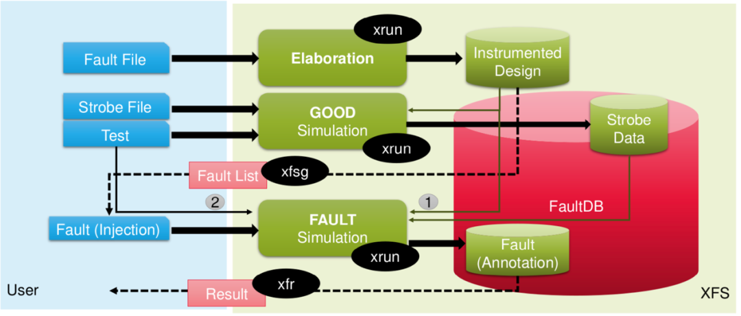
Figure 3.1. XFS Fault Simulation Process
Regarding fault classification, the same method described in Section 2.3.4 is adopted.
It is strongly recommended to encapsulate all necessary commands and their flags and options in a single Make entry using a Makefile. Another advantage of the Makefile is that it allows declaring environment variables when starting new commands. With the Makefile, there is no need to split and rewrite all files for functional verification, FIeVC fault simulation, and XFS fault simulation. By simply wrapping the non-shared code parts with ifdef directives, only the code parts for the required process will be executed.
04. Results
To validate the performance of FIeVC, a small portion of the SMI240 was used as the DUT, specifically the selected part was the accelerometer data path. From the total of 37542 faults in this component, 1000 fault samples (500 SA0 and 500 SA1) were extracted, with each fault point being a driving end to avoid different behaviors when simulating with XFS and FIeVC (see Section 2.6.2). After both simulations ended, a report containing all necessary information was generated.
Figure 4.1 shows a comparison of the classification results from both tools. It can be seen that XFS could only classify 840 out of the 1000 faults, likely because it was unable to inject errors at these points. The 160 un-injected faults are evenly distributed across the other four categories, with the match between UU and DU in both tools being nearly perfect. The only shortcoming of FIeVC is the anomalous behavior observed in the DD and UD classifications, where the tool classified many expected DD errors as UD. The tendency to prioritize UD classification over DD may need to be traced back to the impact of the force command on the system (see Section 2.6).

Figure 4.1. Comparison of Fault Classification between XFS and FIeVC
The key performance indicator (KPI) used to check the consistency between FIeVC and XFS is the test coverage (TC). TC is defined as the percentage of detectable faults in the design that are detected, i.e., the ratio of detected faults to injected faults. This means that if the TC of both tools is similar, their overall behavior can be considered similar.
As expected, both have the same TC, and Figure 4.2 shows a simple comparison between them. More relevant in the figure is the simulation time. As shown, the FIeVC simulation took only 7 hours, while XFS took 22 hours. This means that the time taken for FIeVC to execute a complete simulation was reduced by 68%, which is a significant improvement considering that a complete fault simulation can take weeks or even months. The two main factors contributing to this outstanding performance are the runtime Testflow reset and the parallel algorithm, as previously mentioned.

Figure 4.2. Comparison of TC and Total Simulation Time between XFS and FIeVC
05. Conclusion
This series of articles focuses on the development of fault injection and analysis tools for safety-critical application SoCs, where the impact of faults can be devastating. The environment is developed using the Specman e language and is fully compatible with the underlying verification environment, aiming for non-intrusiveness, ease of use, high adaptability, and flexibility.
The design of this tool is based on the most common fault simulator architecture, with the main components including:
・ A driver for injecting new faults.
・ A monitor for checking whether faults propagate to outputs.
・ An analyzer for classifying each fault.
・ A fault database.
The comparison results with the well-known tool XFS indicate that using parallel algorithms instead of serial algorithms, along with the optimized Testflow reset process, reduced the total simulation time by 68% while maintaining the same level of test coverage. This means that although the two tools are not entirely consistent in fault classification, they yield the same overall analysis results. Furthermore, the threefold performance improvement is crucial in the field of fault simulation, as simulations and analyses can last for days (or even months). The current main limitation of this architecture is the inability to correctly inject all existing fault points due to the internal backward propagation issue mentioned in Section 2.6.2. However, this limitation may be eliminated in the near future by finding methods to prevent backward propagation.
FIeVC has a bright future in BST, but there is still much room for improvement to make it more general and a part of the BST standard verification process. The full potential of this tool can be released in the future through the following directions:
・ Addressing the backward propagation issue.
・ Evaluating the advantages of parallel injection of multiple faulty DUTs to optimize simulation time.
・ Expanding the environment for more complex and precise analyses.
・ Conducting new tests on larger designs (such as system-level architectures) or more complex designs (such as gate-level components) to check whether this tool is applicable in all these different scenarios.
・ Initiating the ISO certification process to ensure the compliance level of this tool and check its applicability for actual application projects for external customers.
Disclaimer: The views expressed in this article are for sharing and communication purposes only. The copyright and interpretation rights of the article belong to the original authors and publishing units. If there are any copyright issues, please contact [email protected], and we will address them promptly.
Related Articles ●●
|Functional Safety Considerations for Basic Steering Systems
|Michelin and Brembo Collaborate to Change Automotive Braking
|US Media: Tesla Cybertruck Issues Continue to Worsen
|Analysis of AUTOSAR Methodology and Technical Implementation
|Safety Architecture for Evaluating Perception Performance of Assisted and Autonomous Driving
|ECU Hardware Design for Functional Safety of Vehicle Network Communication
|ISO 21434 Cybersecurity Engineering Methodology
|Using Fault Injection to Validate AUTOSAR Applications According to ISO 26262
|Achieving Functional Safety ASIL Compliance for Autonomous Driving Software Systems
|Latest Developments: Status of Major Automotive Manufacturing Projects by Ford, GM, and Others in 2025
|Overall Chiplet Solutions for Autonomous Vehicles (II): Communication Solutions