Institute of Robotics Planning and Control—— A comprehensive, professional platform for robotics/autonomous driving planning and control. A WeChat account with 40,000 subscribers. Click the blue text “Institute of Robotics Planning and Control” below the title to follow us for valuable and in-depth reading.
Introduction
Imagine driving at 70 miles per hour on a busy highway when a car suddenly cuts into your lane. In milliseconds, your brain processes visual information, tracks the moving vehicles, and decides whether to brake or steer. Now, imagine building a computer system that is faster, more accurate, and distraction-free.This is what my computer vision system achieves: a real-time collision avoidance system that can track multiple vehicles simultaneously and predict potential collisions before they occur. The system relies on two core computer vision technologies—object tracking and collision detection—but what do these terms actually mean in practice?
Object tracking refers to the process of tracking specific objects (such as cars, pedestrians, or cyclists) across a series of camera images. It’s like closely following a car while weaving through traffic, except the computer tracks multiple objects frame by frame simultaneously. In mass-produced autonomous vehicles, frames are typically captured at a frequency of 10 Hz (10 times per second) to balance safety requirements involving human reactions and computational limitations.
On the other hand, the collision detection system takes this tracking data and poses a critical question: “Based on the movement of these objects, will they collide with us?” These systems combine object tracking with physical calculations to predict potential accidents before they happen, giving the vehicle time to brake, steer, or alert the driver.
In real-world autonomous vehicles, collision detection is extremely complex—I spent a significant amount of time developing this technology during my career at Tesla and General Motors Cruise. Different types of objects (pedestrians, cars, and trucks) are assigned different risk weights. The system considers factors such as collision angles, object mass, distance, and speed, as well as sensor performance degradation. For example, the response triggered when a pedestrian enters the road is vastly different from that of a slowly moving truck.
While production systems typically integrate multiple sensors (cameras, radar, and LiDAR), this project will focus on a camera-based foundational perception process to simplify the workflow. Camera systems provide extremely rich visual information, forming the backbone of visual perception in autonomous vehicles. Complete code and implementation details can be found at https://github.com/moorissa/2D-object-tracking/.
1 Why 2D Tracking is Crucial in a 3D World
One might ask, if we already have LiDAR (Light Detection and Ranging) providing precise 3D measurements, why bother with camera-based 2D tracking? The answer lies in sensor fusion and redundancy—two principles that are essential in safety-critical systems.
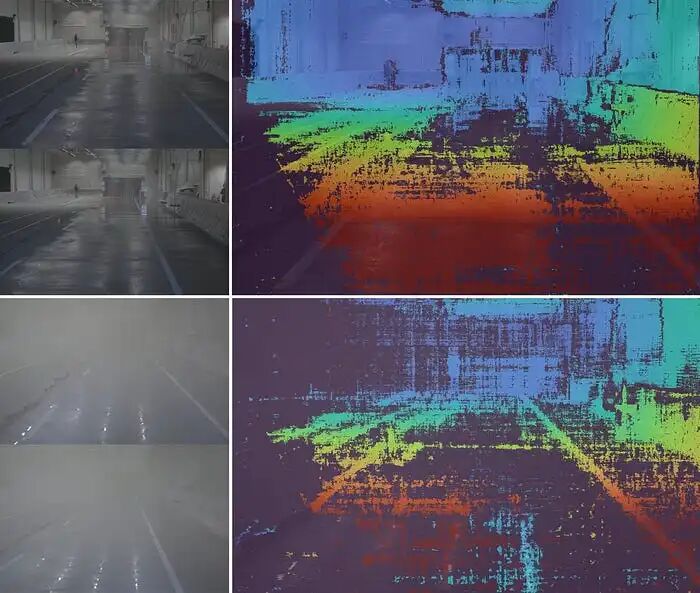
Cameras have unique advantages that are indispensable, just like LiDAR. First, they provide rich visual environments. Unlike LiDAR, which offers geometric accuracy but lacks semantic detail, cameras can capture colors, lane markings, and fine visual cues. This additional information helps the system distinguish between seemingly similar objects. For instance, while LiDAR can detect the geometric shape and position of a traffic light pole, it cannot determine whether the light is red, yellow, or green—critical information for safe navigation.
Cameras are also more cost-effective. High-resolution cameras are significantly cheaper than LiDAR, allowing for broader sensor coverage and more scalable deployment. Additionally, under certain weather conditions, cameras often outperform LiDAR in durability. While radar is the gold standard for extreme weather, cameras tend to maintain clearer performance in heavy rain, snow, or fog.
Another key advantage is computational maturity. The field of computer vision has optimized algorithms for two-dimensional image data for decades, resulting in efficient models that can be deployed on embedded systems with minimal computational load. Compared to processing dense 3D point clouds, camera-based processing is typically faster and less resource-intensive.
Today, camera-based depth estimation technology is rapidly advancing. Companies like Nodar are pushing technological boundaries by converting stereo camera feedback into dense 3D depth maps similar to LiDAR, all based on two-dimensional image data. This technology not only expands the application range of cameras beyond classification but also challenges the notion that 3D perception must come from traditional active sensors. It highlights the importance of camera data in modern autonomous perception stacks.
But perhaps the most compelling reason to retain 2D tracking is that redundancy can save lives. In autonomous driving systems, having multiple ways to detect and track objects means that if one sensor produces unreliable data or fails (due to occlusion, hardware issues, or environmental noise), another sensor can step in. Redundancy is a critical safeguard that determines whether one escapes by luck or faces catastrophic failure. As for cameras, they are not just an enhancement in the 3D world. They are essential for perception robustness, system resilience, and safety.
2 The Pipeline
Building an effective 2D tracking system involves addressing several interrelated issues:
- Feature Detection: Identifying feature points in images that can be reliably found across multiple frames. These feature points may be corners, edges, or texture patterns that differ from the surrounding environment.
- Feature Description: Creating a compact mathematical representation of these points that remains consistent under changes in lighting, rotation, and scale. This can be thought of as giving each feature a unique “fingerprint.”
- Feature Matching: Associating features between consecutive frames to understand the motion of objects. We connect the points (literally!) to track the movement of objects in the scene.
- Performance Optimization: Completing all these operations quickly enough to achieve real-time performance while maintaining accuracy. In autonomous vehicles, there is no room for slow algorithms.
Imagine it like following a friend in a crowded concert. You might track them by their unique red jacket (a “feature”), but what happens when the lighting changes, they turn around, or someone partially blocks your view? Your tracking system needs to be equally adaptive, but it must track dozens of objects and make decisions in an instant.
3 Step-by-Step Implementation
Building this system from scratch made me realize that computer vision requires both mathematical knowledge and engineering pragmatism. Here’s how the process works in practice:
Step 1: Prepare Visual Data
Before any tracking can occur, we need to efficiently process vast amounts of video footage. Our system uses a ring buffer—think of it as a circular conveyor belt that only keeps the latest frames. When a new frame arrives, the oldest frame is automatically discarded. This prevents memory overflow while ensuring we always use the most recent data.
// Ring buffer implementation
dataBuffer.push_back(frame);
if (dataBuffer.size() > dataBufferSize) {
    dataBuffer.erase(dataBuffer.begin());
}
Step 2: Feature Detection Using Keypoints
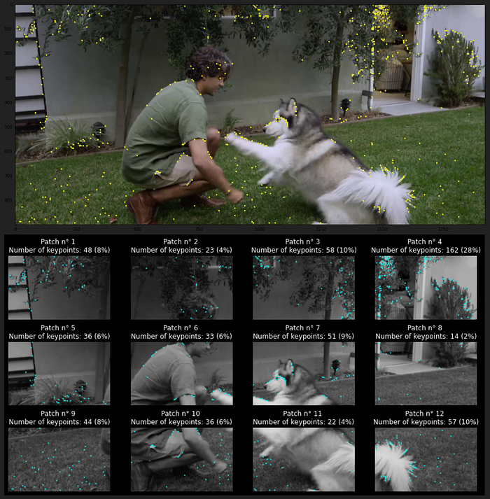
Once we have prepared the frames, the system looks for interesting, unique points. These points are called keypoints. They can be corners of cars, unique patterns on bumpers, or sharp edges. Keypoints help the system ignore visual noise and focus on what truly matters.
For the implementation of the keypoint detector, we used the OpenCV library and compared six different feature detection algorithms—each with its own strengths and weaknesses.
1. HARRIS Corner Detector is considered the pioneer of corner detection. It can find points where image intensity changes significantly in multiple directions. Mathematically elegant, it is computationally intensive and often finds fewer keypoints than modern methods.
// HARRIS Corner Detector: Lines 110-160
void detKeypointsHarris(std::vector<cv::KeyPoint> &keypoints, cv::Mat &img, bool bVis) {
    // Implementation starts at line 111
    cv::cornerHarris( img, dst, blockSize, apertureSize, k );
    // Pixel-by-pixel checking loop at lines 120-140
    for (int i=0; i < img.rows; ++i) {
        for (int j=0; j < img.cols; ++j) {
            float response = dst_norm.at<float>(i,j);
            if ((int) response > threshold) {
                // Create keypoint and handle overlaps
            }
        }
    }
}
2. FAST (Features from Accelerated Segment Test) is very fast but sometimes less accurate. As the name suggests, FAST prioritizes speed. It identifies corner points by checking 16 pixels around each candidate point in a circle. If enough contiguous pixels are significantly brighter or darker than the center, it is marked as a feature.
// FAST: Lines 175-183 (within detKeypointsModern function)
if (detectorType.compare("FAST") == 0) {
    cv::Ptr<cv::FeatureDetector> detector = cv::FastFeatureDetector::create(30, true, type);
    detector->detect(img, keypoints);
}
3. BRISK (Binary Robust Invariant Scalable Keypoints) perfectly combines speed and robustness by using scale-space methods and binary descriptors. It excels at handling scale variations, which is crucial when objects are close to or far from the camera.
// BRISK: Lines 184-193 (within detKeypointsModern function)
else if (detectorType.compare("BRISK") == 0) {
    int threshold = 30;
    int octaves = 3;
    float patternScale = 1.0f;
    cv::Ptr<cv::FeatureDetector> detector = cv::BRISK::create(threshold, octaves, patternScale);
    detector->detect(img, keypoints);
}
4. SIFT (Scale-Invariant Feature Transform) creates detailed mathematical descriptions for each keypoint, making them invariant to scale, rotation, or lighting changes. SIFT is very comprehensive but computationally intensive.
// SIFT: Lines 210-217 (within detKeypointsModern function)
else if (detectorType.compare("SIFT") == 0) {
    cv::Ptr<cv::FeatureDetector> detector = cv::SIFT::create();
    detector->detect(img, keypoints);
}
5. ORB (Oriented FAST and Rotated BRIEF) attempts to combine the speed of FAST with the robustness of SIFT. While versatile and efficient, its robustness is poorer for significant scale changes.
// ORB: Lines 194-201 (within detKeypointsModern function)
else if (detectorType.compare("ORB") == 0) {
    cv::Ptr<cv::FeatureDetector> detector = cv::ORB::create();
    detector->detect(img, keypoints);
}
6. AKAZE (Accelerated-KAZE) uses nonlinear diffusion filtering to find features that are both unique and stable. It is relatively new but performs excellently across various scenarios.
// AKAZE: Lines 202-209 (within detKeypointsModern function)
else if (detectorType.compare("AKAZE") == 0) {
    cv::Ptr<cv::FeatureDetector> detector = cv::AKAZE::create();
    detector->detect(img, keypoints);
}
The above algorithms are implemented under the `detKeypointsHarris` function in src/matching2D_Student.cpp. We tested these keypoint detectors to determine which one was best at finding the most relevant keypoints on vehicles. We found that the BRISK and SIFT detectors excelled at identifying a large number of relevant features on cars.
Step 3: Region of Interest (ROI) Filtering, Focusing Only on Targets
For vehicle tracking, not every pixel is critical. We implemented a Region of Interest (ROI) to concentrate computational resources on areas where vehicles are likely to appear, primarily the road ahead and adjacent lanes.
For example, after finding all keypoints, it directly discards those outside the vehicle’s rectangular bounding box. This not only improves process efficiency but also prevents the system from being disturbed by untracked objects (like distant buildings). In our code example, we use the `.contains` method of the `VehicleRect` object to detect and remove keypoints outside the rectangular range.
// Remove keypoints outside the vehicle bounding box
if (vehicleRect.contains(keypoints[i].pt)) {
    // Keep this keypoint
}
Step 4: Feature Description, Providing a “Fingerprint” for Each Keypoint
Once the system has a clear set of keypoints on the vehicle, it needs to assign a unique “fingerprint” to each keypoint, known as a descriptor. These are mathematical summaries of the area surrounding each keypoint. A good descriptor is robust and does not change significantly even with lighting variations or slight rotations of the vehicle.
We tested various descriptor algorithms, such as BRIEF, ORB, and SIFT. Similar to keypoint detection, the system can be configured to use different methods to see which one performs best.
// BRISK descriptor example
extractor = cv::BRISK::create(threshold, octaves, patternScale);
extractor->compute(img, keypoints, descriptors);
Step 5: Feature Matching to Connect Points Between Frames
With keypoints and their fingerprints, the system can start connecting the points. The matching step involves comparing the descriptors of keypoints in one frame with those in the next frame. This helps the system determine how the vehicle is moving.
To speed up comparisons, we used a special matching technique called FLANN (Fast Library for Approximate Nearest Neighbors) for faster matching over a large number of keypoints. We also implemented a kNN (k-Nearest Neighbors) matcher for more straightforward but potentially slower comparisons.
Brute Force Matching: Exhaustive but thorough
cv::Ptr<cv::DescriptorMatcher> matcher = cv::BFMatcher::create(normType, crossCheck);
matcher->match(descSource, descRef, matches);
FLANN Matching: Fast approximate matching for real-time performance
cv::Ptr<cv::DescriptorMatcher> matcher = cv::FlannBasedMatcher::create();
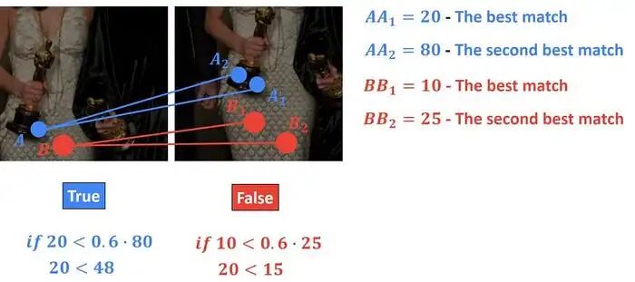
Step 6: Quality Control Using Lowe’s Ratio Test
To eliminate erroneous matches, we applied the ratio test. This test compares the best match with the second-best match—if they are too similar, the match is considered unreliable.
const float threshold = 0.8f;
for (size_t i=0; i < knn_matches.size(); i++) {
    if (knn_matches[i][0].distance < knn_matches[i][1].distance * threshold) {
        matches.push_back(knn_matches[i][0]);
    }
}
4 Results and Evaluation
After comprehensive benchmarking of all detector combinations, several clear patterns emerged, revealing fundamental trade-offs in computer vision system design.
The results of keypoint detection showed significant differences in both quantity and quality among different algorithms. BRISK consistently found the most keypoints, averaging 264-297 per image, providing a rich feature set for robust tracking. SIFT took a different approach, finding fewer keypoints (124-159) but with very high quality and stability across frames. HARRIS generated surprisingly few keypoints (14-43), but these keypoints were often very stable and reliable. FAST was in the middle, with 103-127 keypoints per image while maintaining excellent processing speed.
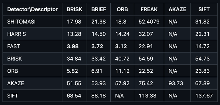
Processing time differences were even more pronounced, revealing the computational costs of complex algorithms. The FAST combination averaged only 3-4 milliseconds to quickly process frames, making it ideal for real-time applications. The ORB combination required 5-11 milliseconds, which is still very reasonable for most use cases. The HARRIS combination took 13-32 milliseconds, reflecting the computational intensity of its corner detection mathematics. The SIFT combination was the slowest, taking 68-137 milliseconds, a significant cost for its superior feature quality.
The success rate of feature matching revealed interesting interactions between detectors and descriptors. The combination with the most matches was BRISK + SIFT, with 1,529 matches; followed closely by BRISK + BRIEF with 1,512 matches, and BRISK + BRISK with 1,426 matches. These results highlight BRISK’s ability to find many trackable features that other algorithms can successfully match. In terms of speed, FAST + ORB had an extremely fast processing speed of just 3.12 milliseconds; FAST + BRIEF had a processing speed of 3.72 milliseconds; and FAST + BRISK had a processing speed of 3.98 milliseconds, demonstrating that speed does not necessarily compromise tracking capability.
The choice of the best combination entirely depends on your system requirements and constraints. For applications requiring the highest accuracy with lower processing time demands, the BRISK detector with SIFT or BRIEF descriptors can provide the highest number of reliable matches, which is crucial for robust tracking under challenging conditions such as weather or lighting changes.
For real-time performance where milliseconds matter, the FAST detector with ORB or BRIEF descriptors can deliver processing times below 4 milliseconds without completely sacrificing tracking quality. For production systems that need to balance reliability and responsiveness, FAST + BRISK offers an excellent compromise with a processing time of 3.98 milliseconds while maintaining strong matching performance.
Winning Strategy
The “best” combination entirely depends on your specific needs. From this exercise, we found that to achieve the highest accuracy, using the BRISK detector with SIFT or BRIEF descriptors can provide the most reliable matches, which is crucial for robust tracking under challenging conditions.
In terms of real-time performance, the FAST detector with ORB or BRIEF descriptors can deliver processing times below 4 milliseconds, which is critical for time-sensitive autonomous driving applications. More complex algorithms like SIFT and AKAZE are much slower.
Overall, to achieve balanced performance, FAST + BRISK provides an excellent balance between speed (3.98 milliseconds) and matching quality, making it an ideal choice for production systems that require reliability and responsiveness.
5 Conclusion
The process of building a vision system often makes me realize the vast gap between academic theory and practical production environments. Computer vision textbooks showcase perfect corner detection examples, but they do not prepare us for the moment when algorithms confidently match branches with car antennas. Real-world feature matching is messy, unpredictable, and full of false positives.
Sometimes, the solution is not a more complex algorithm, but better quality control.
Moreover, there are always real-time performance constraints. For instance, SIFT can generate extremely robust features but takes 40 times longer than FAST. On the other hand, FAST may miss subtle details, but it can make decisions while SIFT is still thinking. In autonomous systems, “good enough and fast” often trumps “perfect and slow” because if it’s too late, perfection is useless and even unsafe.
The initial programming exercises quickly deepened my understanding of how these core perception algorithms apply in real life: they drive the collision avoidance features of ADAS, automated parking, lane keeping, adaptive cruise control, and even optimize traffic flow for smart cities. Every time a car brakes before a collision or stays centered in its lane, you are likely witnessing the practical application of these algorithms!
Beyond the code, I hope this project gives you a clearer understanding of how these core building blocks (such as keypoints, descriptors, and matchers) form the foundation of almost everything in modern perception. Whether you are a student exploring computer vision or an engineer building future autonomous systems, I hope this project lays a solid foundation for your innovations.