Today,the data processing architecture exhibits a “split” characteristic. The focus has shifted to “cloud” computing, which boasts massive scale and computational power, while “edge” computing places the processing right at the “front line”, connecting electronic devices with the real world. In the cloud, the volume of data stored is enormous, and processing must be queued and scheduled; whereas at the edge, processing tasks are completed instantaneously and purposefully.
This enables the system to respond quickly to local instructions and application feedback while reducing data traffic to ensure a more secure processing experience. Of course, these two areas also interact, with edge nodes sending data back to the cloud for cross-device or location aggregation and analysis; while global commands and firmware updates are relayed back to the edge.
Both processing environments benefit from the latest developments in artificial intelligence (AI) and machine learning (ML). For instance, in data centers, thousands of servers containing tens of thousands of processors (mainly GPUs) perform large-scale parallel computations to generate and run large language models (LLMs) like ChatGPT. By some metrics, the performance of these platforms has now surpassed that of humans.
At the edge, the processing responds to feedback sensors and instructions based on operational algorithms. However, with the help of machine learning, algorithms can now effectively learn from feedback; thus improving the algorithms and their computational coefficients, making controlled processes more accurate, efficient, and secure.
Energy Consumption Differences Between Cloud and Edge
In terms of energy usage scale, there are significant practical differences between cloud computing and edge computing. Energy consumption in both scenarios must be minimized; however, the power consumption of data centers is immense. According to the International Energy Agency (IEA), it is estimated to be around 240-340 terawatt-hours (TWh), accounting for 1%-1.3% of global demand. AI and machine learning will further accelerate energy consumption; the IEA predicts a growth of 20%-40% in the coming years, while the historical figure is only about 3%.
Unlike on-demand data processing tasks such as gaming and video streaming, AI encompasses both learning and reasoning stages; the learning phase relies on datasets to train models. Reports indicate that ChatGPT consumed over 1.2 TWh of electricity during this process. On the other hand, according to de Vries’ statistics, LLMs in the reasoning or operational phase may require 564 MWh of power daily.
At the other end of the data processing architecture, edge computing power consumption in IoT nodes or wearable devices may not exceed the milliwatt level. Even for industrial and electric vehicle (EV) applications like motor control and battery management, the reserved power budget for control circuits is minimal, unable to accommodate the significant energy consumption increases brought about by AI and machine learning.
Therefore, tiny machine learning (tinyML) has evolved into an application and technology field for implementing sensor data analysis on devices; it has also been optimized to achieve ultra-low power consumption.
TinyML and Power Management
Implementing machine learning technology in specific applications involves multiple dimensions. For example, tinyML can be used for battery management, aiming to control discharging with minimal stress while charging as quickly, safely, and efficiently as possible. Battery management also monitors the health of the battery and actively balances the cells to ensure even aging for maximum reliability and lifespan.
Monitored parameters include the voltage, current, and temperature of individual cells; management systems typically need to predict the state of charge (SOC) and state of health (SOH) of the battery. These parameters are dynamic quantities, with complex and variable relationships to the battery’s usage history and measured parameters.
Despite the complexity of the task, achieving AI processing does not require expensive GPUs. Modern microcontrollers like the ARM Cortex M0 and M4 series can easily handle machine learning tasks in battery management, and their power consumption is very low, having already been integrated into dedicated system-on-chip (SoC) solutions for this application.
Battery management ICs are quite common, but with the help of MCUs implementing machine learning algorithms, the information and patterns based on historical and current sensor data can be used to better predict SOC and SOH while ensuring high safety. Like other ML applications, this requires a learning phase based on training data; data can come from logs containing different environmental conditions and multiple battery manufacturing tolerances; in the absence of actual field data, synthetic data obtained from modeling can also be utilized.
As is the nature of AI, models can be continuously updated as field data accumulates, allowing for scaling up or down of applications or for use in other similar systems. While the learning process is typically a pre-deployment task, it can also become a background task based on sensor data, processed offline either locally or via the cloud for ongoing performance improvements. Automated machine learning (AutoML) tools combined with battery management SoC evaluation suites can achieve this functionality.
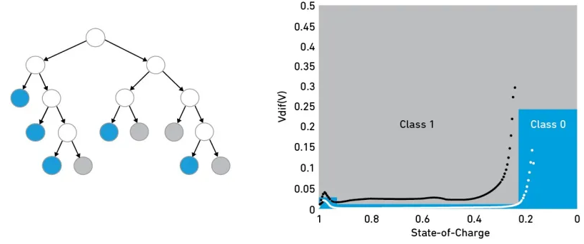
In the field of edge applications like machine learning and battery management, there are various models to choose from. A simple classification decision tree occupies very few resources, requiring only a few kilobytes of RAM, but can provide sufficient functionality for such applications. This method can simply categorize the collected data as “normal” or “abnormal”; an example is shown in Figure 1.
Figure 1: In this decision tree classifier example, “Category 1” = normal, “Category 0” = abnormal
Here, two parameters are used to describe the state during the discharge process of a multi-cell battery pack: the SOC (state of charge) of the strongest cell and the voltage difference between the strongest and weakest cells. The blue and white nodes represent normal data; the classification regions are indicated in blue (“Category 0″= normal) and gray (“Category 1″= abnormal).
If you want to evaluate continuous values of output data, rather than just categories, more complex regression decision trees can be used. Other common ML models include support vector machines (SVM), kernel approximation classifiers, nearest neighbor classifiers, naive Bayes classifiers, logistic regression, and isolation forests. Neural network modeling can be included in AutoML tools to enhance performance at the expense of increased complexity.
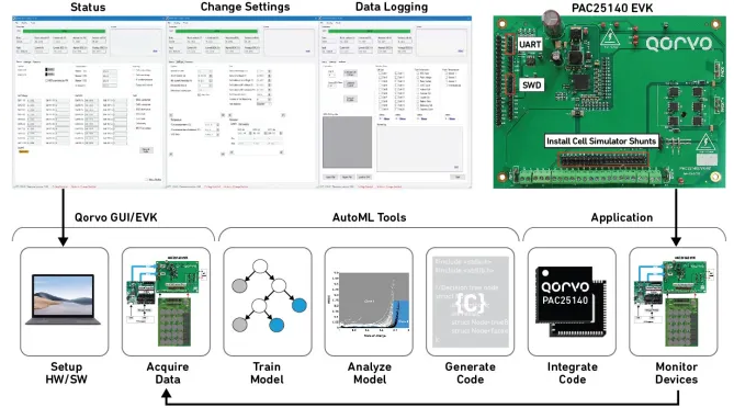
The entire development process of an ML application is referred to as “MLOps”, which stands for “ML Operations”, encompassing data collection and organization, as well as model training, analysis, deployment, and monitoring. Figure 2 graphically illustrates the development process of a battery management application using the PAC25140 chip; this chip can monitor, control, and balance a series battery pack composed of up to 20 cells, suitable for lithium-ion, lithium-polymer, or lithium iron phosphate batteries.
Figure 2: The above design example highlights the tinyML development process
Case Study: Weak Cell Detection
Weak cell detection is part of battery SOH monitoring. One characteristic of these cells may manifest as abnormally low battery voltage under load. However, voltage is also influenced by actual discharge current, state of charge, and temperature, as shown in Figure 3; the figure highlights the example curves of strong and weak cells under different temperatures and load currents.
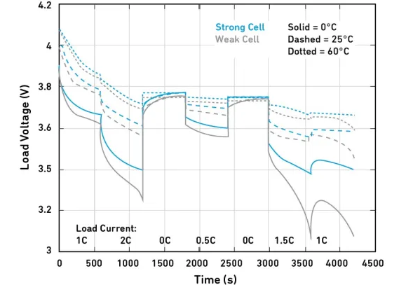
Figure 3: Discharge curves of strong and weak cells
Figure 3 shows the significant voltage differences between strong and weak cells as the cell’s charge approaches depletion; however, detecting a weak cell at this point may be too late to avoid overheating and safety issues. As a result, implementing ML becomes a solution to identify relevant patterns from data at earlier stages of the discharge cycle.
The effectiveness of ML methods is well demonstrated in experiments conducted by Qorvo. The experiment involved inserting a weak cell into a battery pack consisting of 10 cells and comparing it with a well-functioning battery pack. Both sets of cells discharged under different constant current rates and temperatures, generating training data; monitored parameters included their current, temperature, voltage difference between the strongest and weakest cells, and the SOC of the strongest cell.
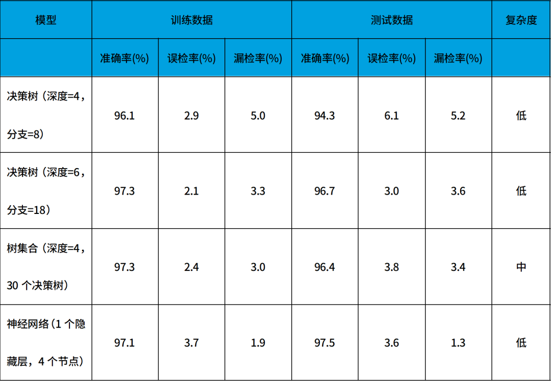
During 20 discharge cycles, parameters were synchronized sampled every 10 seconds and analyzed using different models listed in Table 1. Comparing the results with independent test data from the 20 discharge cycles showed that the consistency of the two methods was very close; as the training samples increased, their consistency would further improve.
Figure 4: Extracted example results from training and testing data of different ML models
SOC Sufficient to Support ML
While the current focus of AI is on large-scale, high-power applications; however, for applications like battery monitoring, using MCU and tinyML technology in an “edge-deployed” AI can also become part of a high-performance, low-power solution. In this scenario, SoC solutions possess all the necessary processing power and can integrate various machine learning algorithms.
All necessary sensors and communication interfaces are built-in; moreover, SoCs are supported by a rich ecosystem of evaluation and design tools.
Paul Gorday is the Director of DSP and Machine Learning Technologies at Qorvo.