Getting Started with TinyML: A Comprehensive Guide

Introduction to TinyML

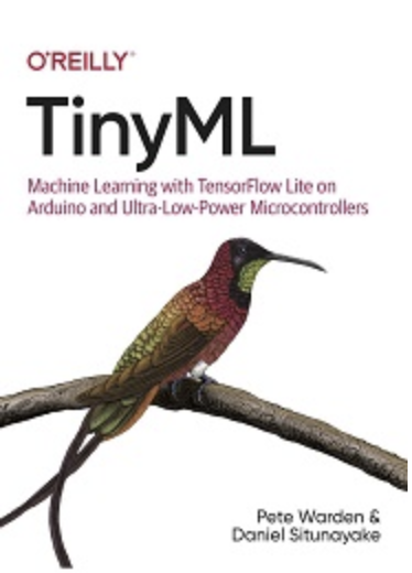
Pete Warden and Daniel Situnayake co-authored a book introducing how to run ML on Arduino and ultra-low-power microcontrollers, TinyML: Machine Learning with TensorFlow Lite on Arduino and Ultra-Low-Power Microcontrollers, published by O’Reilly on December 13, 2019.

As a GDE in both IoT and ML in China, I have been continuously paying attention to the application of AI in embedded systems and the Internet of Things. After hearing about the book’s publication, I couldn’t wait to get a copy of the English version, which I found captivating. I also wanted to prototype how to build a complete engineering process for TinyML and share it with everyone.

Before reading this article, I will briefly introduce TinyML.

Machine Learning (ML) has a history of about 40 years in academia, but the first 30 years only saw some breakthroughs in academic research.

The real milestone that allowed ML to transition from academia to industry was the 2010 ImageNet challenge (ILSVRC). In 2012, the Hiton (an elder in the ML field) research group first participated in the ImageNet image recognition competition, where AlexNet won the championship and outperformed the second place (SVM) in classification performance. The enthusiasm for ML in industrial applications was completely ignited that year.

In recent years, ML has gained a lot of applications in industry and consumer fields, and with the continuous improvement of cloud resources, more exciting AI models have been developed. The application of cloud AI has made significant progress.

During the development of industrial applications of ML in recent years, the Internet of Things has also been rapidly developing. From the early smart home devices to the current widespread IoT smart devices, AI applications are gradually moving from the cloud to the device side, where AI applications on the device side now account for a significant proportion, and AI applications on mobile phones have become very common.

However, in the IoT world, there are billions of small, low-power, resource-constrained devices supporting IoT applications. How to run AI applications on ultra-low-power (mV power range) devices while meeting the demand for long-term low-power operation of AI applications has become a new topic.

TinyML refers to the methods, tools, and techniques for implementing machine learning on microprocessors with mW power. It connects IoT devices, edge computing, and machine learning.

1. The technical hardware for TinyML has reached a practical stage;
2. Algorithms, networks, and ML models under 100KB have made significant breakthroughs;

3. The demand for low-power visual and audio applications is rapidly increasing.

TinyML will achieve faster development in the coming years with the advancement of intelligence. This field also has enormous opportunities.

3. Authors of the Book

Pete Warden was originally the CTO and founder of Jetpac. He officially joined Google in 2014 and is now the technical leader for TensorFlow on mobile and embedded platforms. It should be noted that Jetpac has strong analytical capabilities for social media photos, providing city guide services for travelers. The company was acquired by Google in 2014.

Daniel Situnayake was a Developer Advocate for TensorFlow Lite at Google and has been actively involved in the TinyML community at Meetups. He is also a co-founder of Tiny Farm, the first company in the US to produce insect protein through industrial automation.

One of the authors focuses on AI technology development in IoT, while the other focuses on implementing AI technology for industrialization. Together, they published this book, leading us to further explore all technical aspects of industrial implementation of AI at the IoT end, reflecting the thought process of using Google’s technology to promote development.

4. Development Environment

For the development environment, we only need to connect peripherals via USB on the computer. Of course, depending on each reader’s habits, you can use your preferred compilation tool to compile this environment, and all of this code can run on Windows, Linux, or macOS. Many trained models can also be downloaded from Google Cloud. You can also use Google Colab to run all the code without worrying about having a unique hardware development environment.

I recommend using the Spark Fun Edge development board, which can be purchased for about $15. By the time this book was published, the second version of Spark Fun had already been developed and could support running all example projects. Readers need not worry too much about the hardware version compatibility of the development board.

Of course, there are also two other supported development boards: Arduino Nano 33 BLE and STM32F746G development boards, and developers can choose flexibly according to their needs.

All projects in this book rely on the TensorFlow Lite development framework on microcontrollers, and the required hardware environment only needs around tens of KB of storage space.

• Projecthttps://github.com/tensorflow/tensorflow/tree/master/tensorflow/lite/micro

We also know that for open-source software, due to continuous updates, optimizations, bug fixes, and support for other devices, the code is constantly changing. Perhaps the code examples mentioned in the book may not be entirely consistent with the code on GitHub, but the basic principles are the same.

In software development, we can also choose an IDE development tool that suits us. However, since I (not the original author of the book, but myself) have been using Linux for many years and am a loyal fan of Vim, all the content I will introduce later is based on the Vim + terminal model. If there are any issues related to development tools, feel free to leave a comment at the end of this article, and we can discuss it together. Regarding command execution, we can easily use the terminal in Linux and macOS. In Windows, command line tools can be used to solve development issues.

Another issue in embedded development is the need to communicate with the development board. If using the Spark Fun development board, Python commands are needed for project compilation; if using the Arduino development board, you only need to load the development package in the Arduino development environment.

The general process for deploying a machine learning engineering project is as follows:

1. Define the goal

2. Collect the dataset

3. Design the model architecture

4. Train the model: be aware of various issues caused by overfitting and underfitting

5. Convert the model

6. Run inference

7. Evaluate and troubleshoot

The engineering process is generally deployed based on the above steps. In the next chapter, we will use the classic introduction to any language, “Hello World,” to illustrate the project-based TinyML engineering development process.

Hello World — The Beginning of Dreams (Part 1)

Hello World is the first sentence every programmer learns when entering the programming world. Its significance lies not in inputting a string of characters in a special way, but in using a simple phrase to understand the most basic process and open a door to a new world.

We will divide “Hello World — The Beginning of Dreams” into three parts: Part 1 will teach developers how to build and train models step by step, Part 2 will mainly explain how to create engineering applications, and Part 3 will focus on how to deploy the project to microcontrollers.

Without further ado, let’s dive into Part 1.

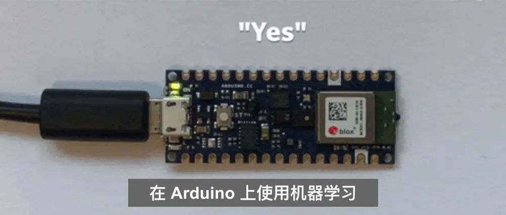
The project can run normally on three different development boards, and we will use Arduino Nano 33 BLE Sense(https://www.arduino.cc/en/Guide/NANO33BLE) as the hardware to implement the ML project based on TensorFlow.

6. Deploy the binary file to the microcontroller

All the code in the article is based on TensorFlow Micro. Of course, the code also includes many comments, and we will analyze the most critical parts of the code and why they are implemented this way.

• TensorFlow Microhttps://github.com/tensorflow/tensorflow/tree/master/tensorflow/lite/micro

The Hello World example we share uses the most basic sine function in mathematics as a prototype to predict data using ML. We have encountered this function when we studied trigonometric functions in middle school. This function is very widely used in industrial applications. A general function graph is shown below:

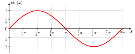
Our goal is to predict the sine value y if we have an x value. In a real environment, using mathematical computation can yield results more quickly. This example uses an ML approach to achieve prediction, thereby understanding the entire ML process.

From a mathematical perspective, the sine function can smoothly oscillate between -1 and 1 periodically. We can use this smooth value to control the brightness of an LED light.

The effect of running this project on the Arduino development board is shown below:

For the development environment, the programming language used is undoubtedly Python, which is the most widely used programming language in science, mathematics, and AI fields. The version is 3.x. Python can run in the command line, but it is still recommended to use Jupyter Notebook for development, as it allows code, documentation, and images to be combined, serving both as a tutorial and enabling step-by-step execution.

If conditions allow, using Google Colab is also a great choice. Colab is a platform developed and maintained by Google, and it has various dependencies already installed on the cloud platform. You can also use Google TPU services for free. Through a web browser, you can run any code you write. You can even use Colab’s configuration files to select accelerated hardware for faster model training.

For the ML platform, there is no doubt that TensorFlow should be chosen, as it is currently the most widely used AI acceleration platform and has a mature pip installation package available. Of course, in the subsequent applications, we will need to use TensorFlow Lite to run the model on embedded hardware, and we will also use TensorFlow’s high-level API, Keras, to complete some programming tasks.

Project-related code:

• https://github.com/tensorflow/tensorflow/blob/master/tensorflow/lite/micro/examples/hello_world/create_sine_model.ipynb

Of course, if running the project on Google Colab, you can run it directly.

We will run our code locally in Jupyter notebook. I downloaded all the source code of TensorFlow using git clone and operated it from the local Linux command line. Since my operating environment is Linux, where all the dependencies are already installed, the code related to pip installation and apt installation in the Jupyter environment has been commented out.

First, run Jupyter:

After starting, a Chrome browser will pop up, as shown in the image:

It should be noted that in the upper right corner, if it prompts as untrusted, click the “untrusted” text and follow the prompts to operate, so that the text will finally change to “trusted.” If the upper right corner indicates that the Python version is 2, then in the Jupyter menu bar, select Kernel > Change Kernel to choose Python 3.

Of course, the first step in the code is to import TensorFlow, Numpy, Matplotlib, and Math libraries. Numpy is used for data processing, while Matplotlib is used for data visualization.

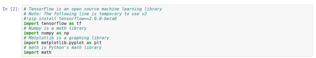
In fact, in the code, I commented out the line #!pip install tensorflow==2.0.0-beta0 because my PC has already installed the latest version of TensorFlow.

First, we will generate a series of standardized data based on the sine function.

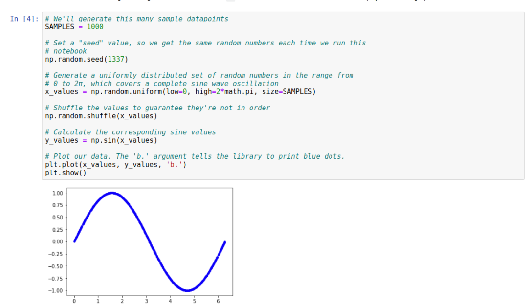
As can be seen, after running, the data is quite standardized. The author has provided some explanations for this segment of the code to help everyone understand the code in detail. Of course, when processing data, Numpy is an optimal mathematical processing function library. The line x_values = np.random.uniform(low=0, high=2*math.pi, size=SAMPLES) is used to generate a series of random numbers within a specific range.

Once the raw data is generated, the next step is data cleaning. We need to ensure that the data reflects in a truly random manner. Fortunately, Numpy’s radom.shuffle() provides such a method.

Finally, we will plot the data in a two-dimensional coordinate system.

This beautiful data can be directly used for training, right? Of course, there’s no problem, but what does ML do? It filters data from various noises, and through training, the prediction accuracy increases. The first operation we need to do is to add some noise. This is also a common method in machine learning. When the samples are insufficient, how do we increase the number of samples to achieve higher accuracy during training?

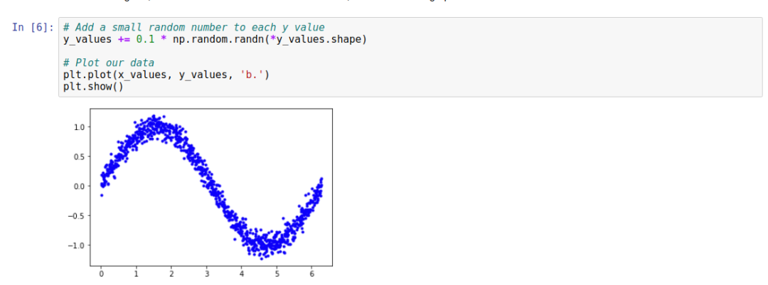
We have completely created all the data.

The next step is to split it into training and testing sets:

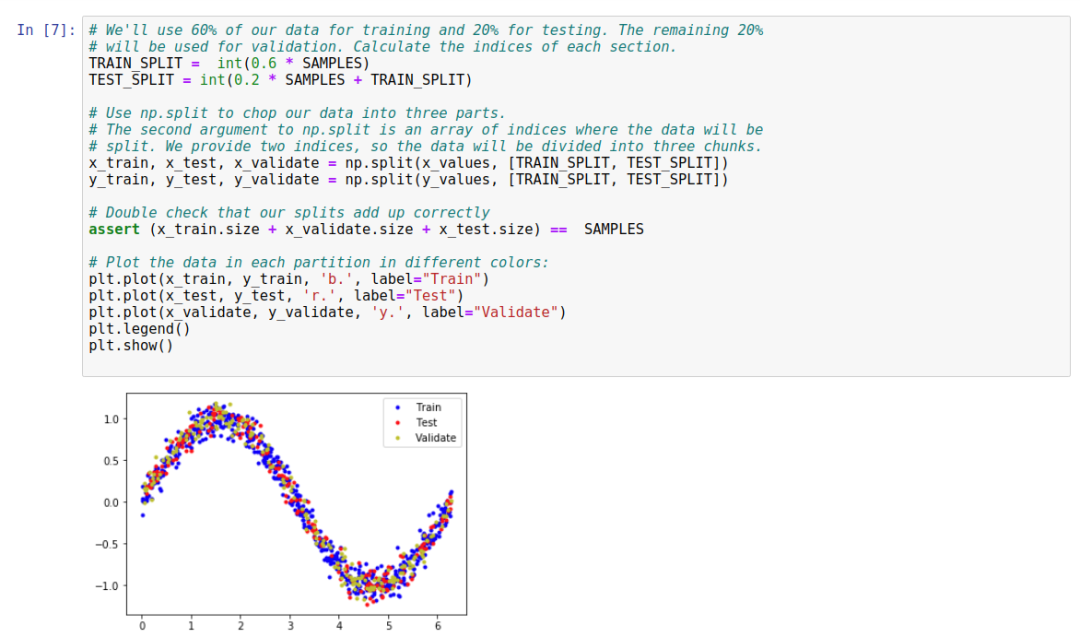
Let’s explain the key code for this part in detail:

TRAIN_SPLIT =  int(0.6 * SAMPLES)
TEST_SPLIT = int(0.2 * SAMPLES + TRAIN_SPLIT)

The entire dataset consists of three parts: training set, testing set, and validation set. In the example, 60% of the data is used as the training set, 20% as the testing set, and 20% as the validation set. This ratio is not fixed and can be adjusted according to requirements.

x_train, x_test, x_validate = np.split(x_values, [TRAIN_SPLIT, TEST_SPLIT]) Although the input parameters only include the training and testing parts, since the entire dataset is divided into three parts, the return result of np.split is three, representing our three scenarios.

6. Defining the Basic Model

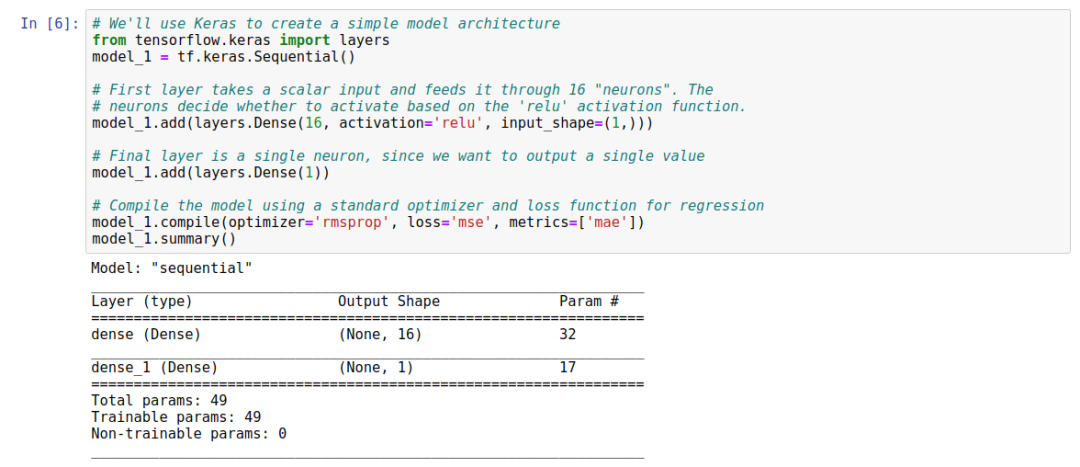
We will use Keras to build the initial model.

The first layer uses scalar input and is based on the “relu” activation function, utilizing a dense layer with 16 neurons. When making predictions, it is one of the neurons in the inference process. Each neuron will then be activated to a certain extent. The activation amount of each neuron is defined by the weight and bias values obtained during training. The activation of the neurons will be output as a number. The activation is calculated through a simple formula, as shown in Python. We will never need to write this code ourselves, as it is handled by Keras and TensorFlow, although understanding the calculation formula’s pseudocode will be helpful during deep learning:

activation = activation_function((input * weight) + bias)

To calculate the activation level of a neuron, the input must be multiplied by the weight, and the bias is added to the result. The computed value is passed to the activation function. The result is the activation of the neuron. An activation function is a mathematical function used to shape the output of a neuron. In our network, we use the Rectified Linear Unit (ReLU) activation function, which is specified in Keras by the parameter activation = relu. ReLU is a simple function, as shown in Python:

def relu(input):
    return max(0.0, input)

ReLU returns larger values: if its input value is negative, ReLU returns zero. If its input value is greater than zero, the output remains unchanged.

What is the significance of using ReLU as the activation function?

Without an activation function, the output of the neurons will always be a linear function. This means that the network can only model linear relationships, where the ratio of x to y remains constant across the entire value range. However, the sine wave is nonlinear, which would prevent the network from modeling our sine wave. Since ReLU is nonlinear, it allows multiple layers of neurons to work together and establish complex nonlinear relationships where each increment of x does not cause y to increase in the same way. There are other activation functions, but ReLU is the most commonly used. As an ML algorithm, using the optimal activation function is essential.

Since the output layer has a single neuron, it will receive 16 inputs. As this is our output layer, we do not specify a definite activation function—we only need the raw result. Since this neuron has multiple inputs, each neuron has a corresponding weight value. The output of the neuron is calculated through the following formula, as shown in Python, where “inputs” and “weights” are both NumPy arrays, each with 16 elements:

output = sum((inputs * weights)) + bias

By multiplying each input with its corresponding weight and summing the results, then adding the bias of the neuron, we obtain the output value. The weights and biases of the network are learned during training.

Next, the key point in the compilation phase is the loss function of the optimizer.

model_1.compile(optimizer='rmsprop', loss='mse', metrics=['mae'])

There are many choices for optimizers, loss functions, and metrics; we will not elaborate on them here. You can go to the following links for more information.

• https://keras.io/optimizers/

• https://keras.io/losses/

Finally, let’s take a look at the model summary:

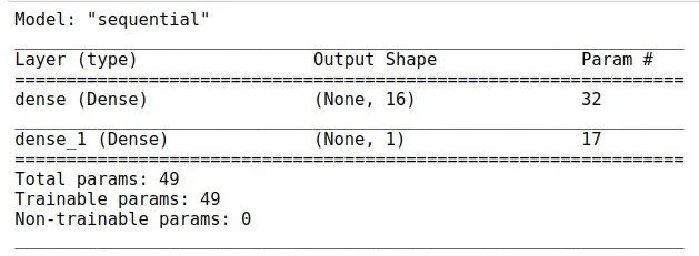
The input layer has 16 neurons, with a total of 2 layers connected, resulting in a total connection count of 16×2=32, and each neuron has a bias, so the total number of biases is 17. The total parameters are 32+17=49.

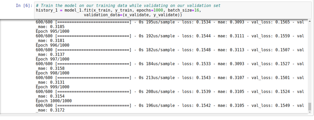
7. Training the Model

• X_train, y_train represent the basic training data.
• epochs indicate the number of training cycles; generally, the longer the epochs, the more accurate the training. However, once the training reaches a certain stage, the training accuracy will not differ much. In such cases, model optimization should be considered.

• batch_size indicates how much data to send into the network at once. If the value is 1, we will update weights and biases with each iteration and estimate the loss of the network prediction for a more accurate estimate in the next run. A smaller value will lead to a significant computational load and consume more computational resources. If we set the value to 600, we can calculate more data at once, but it will reduce the model’s accuracy. Therefore, the best approach is to set the value to 16 or 32. This value selection is actually a trade-off between accuracy and time spent.

Next, we are most concerned about the training results.

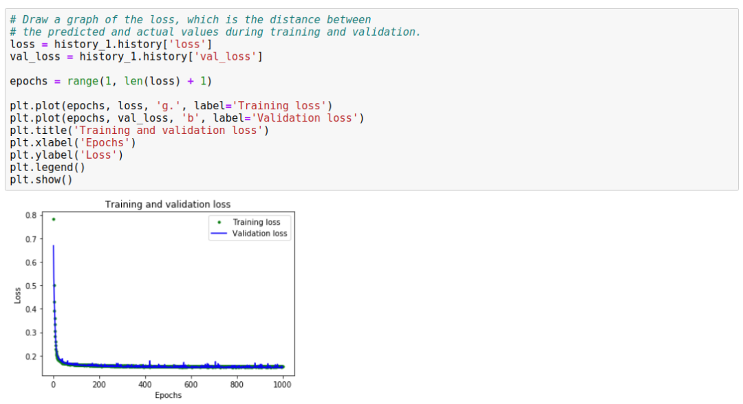
This graph shows the loss for each epoch (or the difference between the model’s predictions and actual data). There are several ways to calculate loss, and we use mean squared error. There are significant loss values for both training and validation data.

We can see that the loss value decreases rapidly in the first 25 epochs and then stabilizes. This means that the model is improving and producing more accurate predictions!

Our goal is to stop training when the model no longer improves or when the training loss is less than the validation loss, indicating that the model has learned to predict the training data well and does not require new data to improve accuracy.

To enhance the readability of the flat portion of the graph, we use the code SKIP = 50 to skip the first 50 epochs, simply for our convenience in viewing the graph.

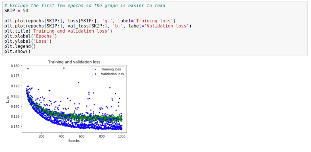
From the graph, we can analyze that around 600 epochs, the training begins to stabilize. This indicates that our epochs do not need to exceed 600.

However, we can also see that the lowest loss value remains around 0.155. This means that our network’s prediction has decreased by about 15%. Additionally, the validation loss shows significant fluctuations and instability. We need to improve our approach. This time, we will plot the mean absolute error (MAE) graph, which is another way to measure the distance between the network’s predictions and actual numbers:

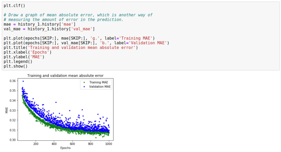
From the mean absolute error graph, we can see that the training data consistently shows lower errors than the validation data, indicating that the network may be overfitting (Overfit) or excessively learning the training data, rendering it ineffective in predicting new data.

Moreover, the mean absolute error value is very high, reaching up to about 0.305, indicating that some predictions of the model can be reduced by at least 30%. A 30% error means we are far from accurately modeling the sine wave function.

This graph clearly shows that our network has learned to approximate the sine function in a very limited way. Starting from 0 <= x <= 1.1, the line fits best, but for our other x values, it is at best a rough approximation.

The results indicate that the model lacks sufficient capability to learn the full complexity of the sine wave function and can only approximate it in a simplistic manner. By optimizing the model, we should be able to improve its performance.

8. Optimizing the Model

The key to optimization is to increase the fully connected layers, which contain 16 neurons.

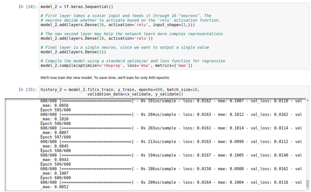
We will then evaluate the model:

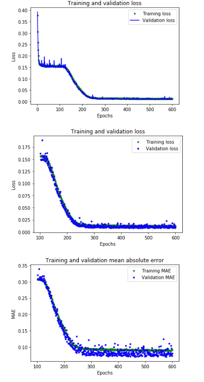
From the image analysis, our network has reached peak accuracy much faster (within 200 epochs instead of 600 epochs). The total loss and MAE are much better than our previous network. The validation results are better than the training results, indicating that the network is not overfitting. The reason the validation metrics outperform the training metrics is that the validation metrics are calculated at the end of each epoch, while the training metrics are calculated over the entire epoch.

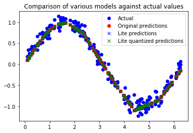
All of this indicates that our network seems to be running well! To confirm this, let’s check its predictions against the test dataset we previously set aside:

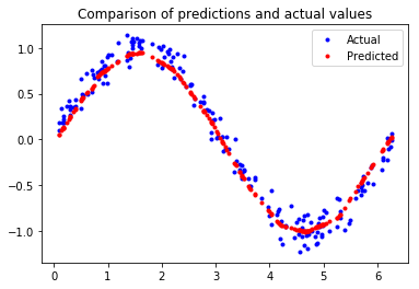
The final test results are shown below:

Looking at this image, it does not indicate that the predicted values perfectly match the sine curve. However, the prediction accuracy is no longer the main issue; we only want to control the switch through a smooth curve. The model’s accuracy is sufficient.

9. Model Conversion

The key point of model conversion is the conversion from TensorFlow to TensorFlow Lite. There are two main components:

This converts the TensorFlow model into a special format that saves space for memory-constrained devices and can further reduce and optimize the model size for faster operation on small devices.

This runs the appropriately converted TensorFlow Lite model on the given device in the most efficient manner.

Similarly, we do not need to operate, but we need to understand the convert Python API and create FlatBuffer, and of course, quantization, which is the issue of converting floating-point precision. Topics like these have been detailed in my previous offline shares about TensorFlow Lite.

The complete conversion code is as follows:

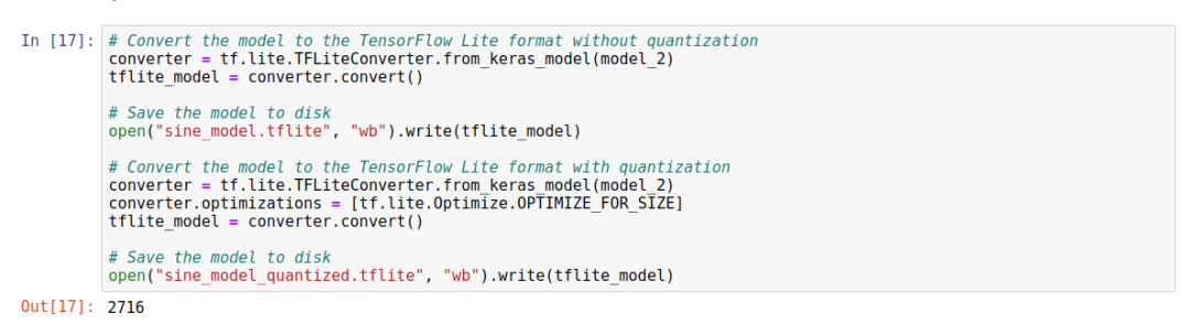
Two models were generated: the first model is unquantized, and the second model is quantized.

1. Declare the interpreter object entity
2. Allocate memory for the model
3. Load the model

4. Read output data from the sensor

Since this segment of code is relatively lengthy, let’s take a look at the final analysis results:

Now let’s compare the size difference between the quantized and unquantized models using code:

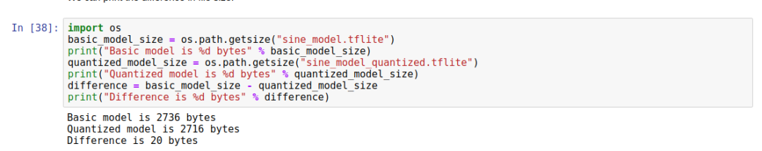
The difference is 20 bytes.

The final step in preparing the model for TensorFlow Lite for Microcontrollers.

So far, in this chapter, we have been using the TensorFlow Lite Python API. This means we can load the model file from disk using the Interpreter constructor. However, most microcontrollers do not have a file system; even if they do, the additional code required to load the model from disk would waste space. Instead, as an elegant solution, we provide the model in the C source file, which is included in our binary file and directly loaded into memory.

In the file, the model is defined as a byte array. Fortunately, there is a Unix tool called xxd that can convert a given file into the required format.

The following output is from running xxd on our quantized model, writing the output to a file named sine_model_quantized.cc and printing it to the screen:

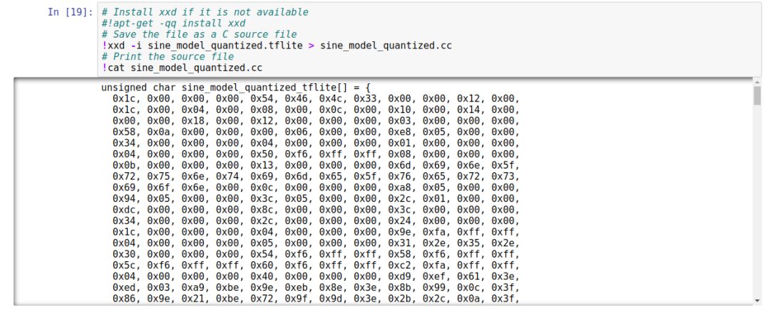
Finally, the work of generating binary model code is completed.

11. Conclusion

Thus, we have completed the model construction. We have trained, evaluated, and configured a TensorFlow deep learning network that can take numbers between 0 and 2π and output approximate sine values.

This is our first experience training a small model using Keras. In future projects, we will train models that are still small but much more complex.

In the next article, we will analyze how to write ML applications that can run on microcontrollers.

— Recommended Reading —