Learning TinyML From Scratch: Optimization Techniques

5. Optimization

Let’s not rush to see what optimization methods this book introduces; let’s carefully review which aspects of optimization we encountered in previous projects.

1. Requirements Analysis and Product Design: Defining the scope of product use. The agreements on the input and output of the product direction will greatly affect the product’s performance. Once the product’s requirements are finalized, we must analyze the specific content of the inputs and outputs and what impact they will have. Data input and output influence the selection of embedded hardware and ML model selection. These factors must be fully considered in the early stages of engineering design.
2. ML Model: After solving the input and output issues, the next step is model establishment and optimization. This part of the content is a well-known topic in machine learning, but it is a necessary consideration in every specific project implementation. The optimization of AI models in embedded systems has been quantified, with methods such as mobile optimization interpreters and hardware acceleration. Much work has been done in optimizing models related to mobile phones, but some new methods have been proposed for optimizing models on microcontrollers. This part of the methods will also be our main discussion direction.
3. When developing any system based on low power hardware, the primary concern is power consumption. Different hardware configurations and the operational characteristics of the system on a chip will have completely different impacts on power consumption. It is particularly important to note that low-power designs may lead to performance losses, so our optimization methods must consider a balance between power consumption and performance; this is the most typical optimization scenario in engineering, where different implementations will yield completely different results.

4. Due to the particularly small storage capacity of low-power microcontrollers, continuously reducing the model size is also a direction for optimization. With these constraints in place, we must evaluate whether the model is optimized from various aspects such as system limitations, memory, storage, and operational efficiency. Evaluation methods for model optimization in similar scenarios need to be continuously explored. There is no best, only better.

Through the analysis of the above elements, we find that engineering optimization is not just about providing the fastest running model; it also involves many other considerations. This time, we will focus on how to optimize on low-power microcontrollers.

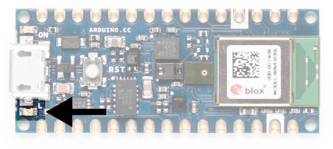
Since the book discusses many directions for optimization, we will divide the specific contents of optimization into two main parts: model optimization, which mainly discusses how to determine product requirements and the main methods used to achieve overall model optimization; and engineering optimization, which mainly discusses the issues to consider when the model is imported into low-power microcontrollers.

Optimization in product design, strictly speaking, does not fall within the realm of technical optimization, but it directly affects the overall operational efficiency of the engineering process. This part cannot be evaluated using particularly good technical methods for the model, but there is indeed a significant difference during the phase of capturing engineering requirements for different products.

• Image: The application field of TinyML is on low-power microcontrollers, but if we add cameras to collect data, power consumption will be an important consideration. The startup time of a camera takes at least a few seconds, and the startup will bring significant instantaneous current, and the camera cannot be in a constantly on mode. The frequent switching of the camera between on and off will lead to substantial power loss. The power consumption will vary with different resolutions when capturing images. The way sampling frequency is set also significantly affects power consumption. From this perspective, the selection of the camera directly determines the direction of optimization.
• Sound: The hardware related to sound has similar issues to that of image hardware, but we need to note that with the addition of microphone arrays, although the model can better analyze raw sound data, the power consumption will be higher from a hardware usage perspective.

• Data: The data referred to here is the data reported by some sensors. Since the power consumption of sensors has already been made very low, the optimization direction is still related to sampling frequency. How to ensure the model inference runs at the best time?

Thus, if we need to lead the design and development of a low-power embedded AI product, we need to consider the performance of the microcontroller, data collection terminals, sampling time, and sampling frequency constraints. Moreover, based on the above constraints, we need to customize the AI model.

In the past, we would use the most resources and the best environment to develop the optimal model. However, in the operating environment of models based on low-power microcontrollers, we no longer emphasize that the model must be the best, but rather a compromise between speed and efficiency. As long as the final inference result is within an acceptable range, it is sufficient.

Once we have adjusted and optimized the model, we need to evaluate the latency of the ML model. Since low-power microcontrollers do not have hardware support for floating-point units, evaluating the number of floating-point operations in the ML model and using quantization methods to reduce the execution time of floating-point operations has become a good method for running quantized ML models on microcontrollers for inference. Since most calculations in neural networks are matrix multiplication operations, we can approximate the number of floating-point operations (or FLOP) required for a single inference run. For example, the number of FLOP required for fully connected layers equals the size of the input vector multiplied by the size of the output vector. We can also estimate the FLOP value from papers discussing model architecture. By using this method, we can fully estimate the floating-point operations or the time loss caused by operations after quantization, and then optimize the most time-consuming code to achieve lower latency.

In recent years, there have been many optimization achievements regarding the application of TensorFlow on embedded processors. The optimizations for TensorFlow Lite include the following aspects: quantization, FlatBuffer, mobile optimization interpreters, and hardware acceleration. For TinyML, the main focus is on software optimization.

Taking quantization as an example, the core of quantization lies in using the loss of precision to exchange for running speed, so balancing the relationship between precision and efficiency becomes the core issue in quantization optimization. Since the quantization process occurs after the entire model has been established, for weights, it can be converted using the correct scaling factor. However, for activations, it is trickier because it is unclear what the actual range of each layer’s output is based on model parameters and connection layer inspections. If the chosen range is too small, the output will be clipped to the minimum or maximum value; however, if the chosen range is too large, the output’s precision will be less than its possible precision, risking the overall result’s accuracy. Now the converter provides a representative_dataset() function, which is a Python function that generates the input needed for estimating the activation range, allowing for better optimization.

For different hardware, I sometimes specifically look at optimization methods that certain hardware instructions can provide. This method may lack universality, but it is still quite important for accelerating the model of a single product. However, the troublesome issue is that it requires understanding whether the CPU has special function support and whether the compiler has specifically optimized these instructions. It may even involve the unpredictable method of incorporating inline assembly to support this, which has exceeded the conventional optimization scope.

From these methods, we can see that optimization based on microcontrollers emphasizes whether there is room for hardware optimization.

When choosing hardware, it is best to select hardware that supports TinyML, as this will ensure that the hardware drivers have complete support and that optimization for the development board has been sufficiently done.

Low-power microcontrollers typically use batteries as power sources. Sleep mode is an important factor; reasonable design can greatly extend battery life. We can design sleep and wake-up times based on the hardware duty cycle. The factors of sensor sampling frequency, time, power consumption, etc., have already been elaborated in the product design optimization section, and many compromises need to be made, but they are also within the scope of hardware optimization.

Cascading design is another good consideration. Compared to traditional procedural programming, a major advantage of machine learning is that it can easily scale up or down the number of required computing and storage resources, and accuracy typically decreases moderately. This means that model cascades can be created. For example, if the hardware computing capacity of Level 1 cannot meet our requirements, we will actively activate Level 2 overhead, allowing us to achieve precise results in a shorter time.

Regardless of the platform chosen, Flash and RAM may be very limited. Most microcontroller-based systems have less than 1 MB of read-only storage in Flash, with the minimum being tens of KB. RAM is similar: very few have more than 512 KB of static RAM (SRAM). TinyML can operate with less than 20 KB of Flash and 4 KB of SRAM, but you will need to carefully design your application and engineering to maintain a low footprint.

Most embedded systems have an architecture where programs and other read-only data are stored in Flash and only written when loading new executable files, using it as read-write memory. This technology is similar to the caching techniques used on large CPUs, allowing for quick access to reduce power consumption, but with limited size. More advanced microcontrollers can use power-hungry but scalable technologies like dynamic RAM (DRAM) to provide a second layer of read-write memory. Thus, the number of peripheral read/write operations directly affects operational efficiency.

The usage rate of Flash is also a consideration. Analyzing the efficiency of various segments in the ELF file and optimizing useless code and precompiled optimizations can save a significant amount of Flash space.

RAM optimization mainly includes considerations during both compile-time and run-time. The core runtime applications of ML frameworks do not require large memory, and their data structures should not exceed a few kilobytes in SRAM. These are allocated as part of the classes used as interpreters, so whether your application code creates them as global or local objects will determine whether they reside on the stack or in general memory. We generally recommend creating them as global or static objects, as insufficient space can lead to errors during linking, while stack-allocated local variables may cause runtime crashes. Therefore, the design of the stack and the application’s memory residency space should have a good design scheme before program compilation.

Optimization of binary size is an important aspect of space optimization. Measuring how much space TensorFlow Lite occupies is crucial. The simplest method is to comment out all calls to the framework (including creating OpResolvers and interpreter objects) and then check how much smaller the binary file has become. If similar content is not seen, check again to see if all references have been captured and if there are unnecessary references. The linker will remove all code that is never called and delete it from the package. Reducing code coupling and following programming norms will affect the final size of the generated binary file.

This part of the discussion involves hardware selection issues and various parameter limitations on hardware. From the compilation perspective, especially from the optimization directions during the compilation stage, linking stage, and code execution stage, this optimization process is tailored to create effective tools.

So far, this series of articles has been completely shared. From this series of articles, we have understood the role of TinyML, implemented a project based on TinyML by referring to the source code in the project example, and finally learned engineering optimization methods by analyzing the project development process and focus points. However, the content introduced in this TinyML book goes far beyond this; it also includes some more complex examples and analyses, including principled explanations of some optimization methods. If you are interested in this direction, hurry up and buy this book to read!