Click on the "Xiaobai Learns Vision" above, select "Star" or "Top"
Important content delivered in real time

Author丨Rustle@ZhihuSource丨https://zhuanlan.zhihu.com/p/59640437Editor丨Jishi Platform

Introduction

This article systematically explains the concepts related to edge detection algorithms, supplemented with a large number of diagrams and formulas to help everyone understand various edge detection operators in depth.

Before We Begin:

This article is relatively long, using a lot of diagrams and formulas to help everyone understand various edge detection operators in depth. I hope everyone can read it through. The testing compiler is Matlab, which is a very user-friendly and simple tool for beginners in the field of Computer Vision. It comes with various advanced library functions, making implementation very quick and is more inclined towards experimental applications. Alright, without further ado, let’s take a look at today’s topic – Edge Detection.

1. Introduction

First, let’s briefly understand what Digital Image Processing is, and look at the two main application areas of digital images:

1. Improve the graphical information for human interpretation;

2. Process image data for storage, transmission, and representation, facilitating automatic understanding by machines.

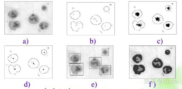
We can simply understand that it transforms a raw image into a form that is more understandable or needed by us. As shown in Figure 1-1, it illustrates the automatic segmentation process of immune cell images based on edge detection.

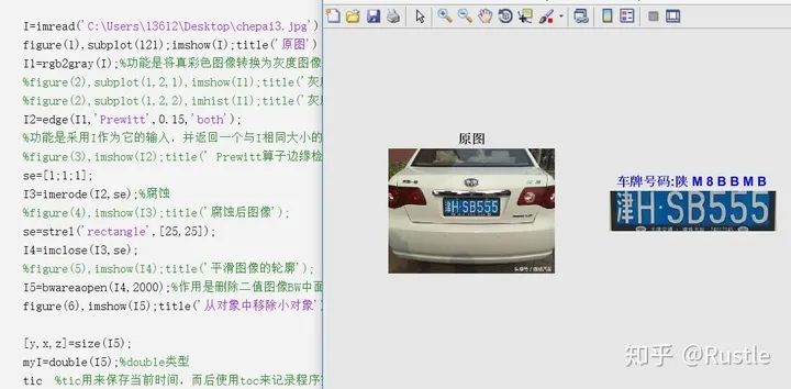
Let’s look at another example, as shown in Figure 1-2, which is a classic License Plate Detection algorithm. It processes the raw image through grayscale conversion, edge detection, morphological erosion and dilation, to obtain the license plate area, and then cuts the license plate area (this is a small demo I did when I first started, and I didn’t use a deep learning model; I used KNN, so the recognition result was poor; I hope the viewers can just smile at this).

OK, after we have a rough understanding of digital image processing, let’s introduce some basic algorithms of digital image processing.

2. Basic Knowledge and Algorithms of Digital Image Processing

Next, let’s briefly introduce some basic knowledge and algorithms for learning digital image processing.

1). Digital Image

A digital image refers to an image represented by two-dimensional numbers, where the grayscale value of each pixel is represented by a number, ranging from 0 to 255 (2^8).

2). Binary Image, Grayscale Image, Color Image

Binary Image: Each pixel’s grayscale value can only be 0 or 1, meaning it is either black or white; a binary image can be understood as a black-and-white image.

Grayscale Image: Each pixel can be represented by a grayscale value of 0-255, specifically represented by 255 intermediate gray values between pure black and pure white.

Color Image: Each image is composed of three grayscale images, representing the grayscale values of the red, green, and blue channels, known as RGB. At this point, a color image is viewed as three-dimensional [height, width, 3].

Below is a diagram to feel the connection and difference between grayscale images and color images.

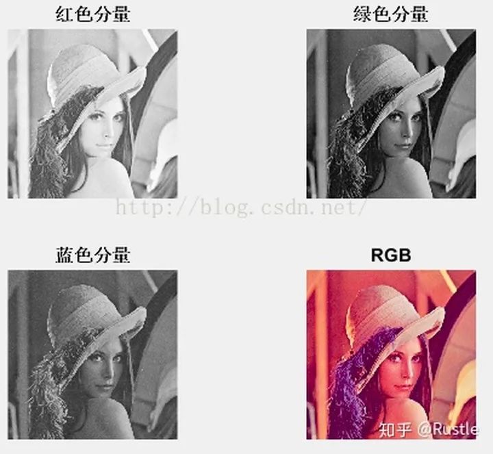
There is also an important formula, which is the calculation formula for converting color images to grayscale images:

G

Gray represents grayscale images, while RGB represents the grayscale values of the red, green, and blue channels of the color image.

3). Adjacency and Connectivity

4-neighborhood: Assuming there is a pixel p with coordinates (x, y), its 4-neighborhood is (x + 1, y), (x – 1, y), (x, y + 1), (x, y – 1).

D-neighborhood: Assuming there is a pixel p with coordinates (x, y), its D-neighborhood is (x + 1, y + 1), (x + 1, y – 1), (x – 1, y + 1), (x – 1, y – 1).

8-neighborhood: The union of the 4-neighborhood and D-neighborhood.

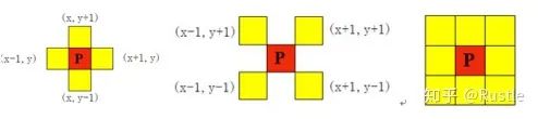
Figure 2-2 4-neighborhood (left), D-neighborhood (middle), 8-neighborhood (right)

4-connectivity: Pixels in the 4-neighborhood of pixel p are all 4-connected to pixel p.

8-connectivity: Pixels in the 8-neighborhood of pixel p are all 8-connected to pixel p.

4). Filtering

The main purposes of filtering are two:

1. To extract image features through filtering, simplifying the information carried by the image for subsequent image processing.

2. To eliminate noise mixed during the digitization of the image through filtering to meet the needs of image processing.

The first point is the basic idea used in edge detection, which is to simplify image information and use edge lines to represent the information carried by the image.

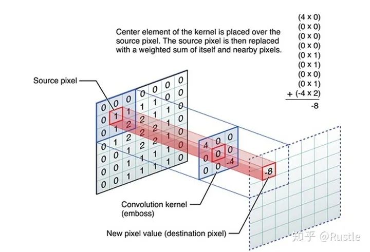
Filtering can be understood as a filter (usually a 3*3 or 5*5 matrix) traversing the image from top to bottom and left to right, calculating the value of the filter with the corresponding pixel and performing numerical calculations to return the value to the current pixel point, as shown in Figure 2-3. The blue block represents the filter, performing dot product operations and assigning values to the image.

The specific formula is represented as:

(where represents the current pixel point, represents the value multiplied by the corresponding value of the filter, and n is the size of the filter. For example, if this filter value is all 1, then this formula calculates the average value of the 8-connected pixels of the current pixel point, so the filtered image should show a blurry effect. The degree of blurriness depends on the size of the filter; the larger the filter size, the more obvious the blurriness).

3. Edge Detection (Sobel, Prewitt, Roberts, Canny, Marr-Hildreth)

1. Basic Edge Detection Operators

After introducing the knowledge of filtering, learning basic edge detection algorithms becomes an easy task because edge detection is essentially a filtering algorithm, with the distinction being the choice of filter; the filtering rules are completely consistent.

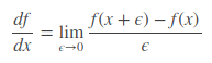
To better understand edge detection operators, we introduce the concept of gradient. The gradient is a very important concept in artificial intelligence, prevalent in the fields of machine learning and deep learning. Those who have studied calculus should know that the first derivative of a one-dimensional function is defined as:

As mentioned earlier, image filtering is generally performed based on grayscale images, so the image is two-dimensional at this point. Let’s take a look at the partial differential equation for the two-dimensional function:

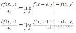
From the above formula, we can see that the image gradient is the partial derivative of the current pixel point with respect to the X-axis and Y-axis, so in the field of image processing, we can also understand the gradient as the rate of change of the pixel grayscale value. Below is a simple example:

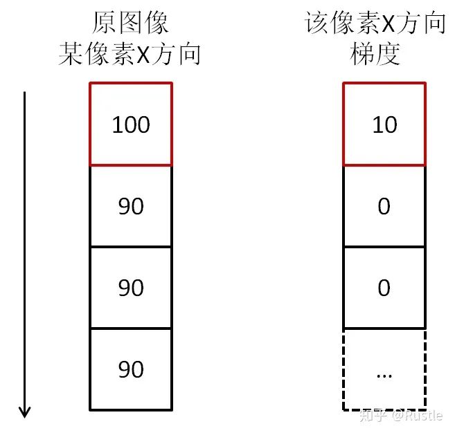
In the figure, we can see that the grayscale value difference between 100 and 90 is 10, meaning the gradient in the X-axis direction at the current pixel point is 10, while all other points are 90. Thus, after differentiation, the gradient is found to be 0. Therefore, we can see that in digital image processing, due to the special nature of pixel properties, calculus manifests itself as calculating the difference along the direction of partial differentiation at the current pixel point, so in practical applications, there is no need to use differentiation; simple addition and subtraction are sufficient.

Another concept, the magnitude of the gradient, represents the amount of increase in the direction of maximum change of f(x, y) per unit distance, i.e.:

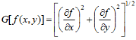
After understanding the concept of gradients, let’s first introduce a few basic edge detection filters: Sobel, Prewitt, and Roberts operators.

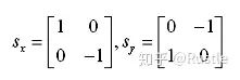
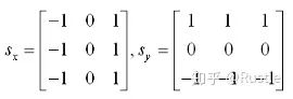
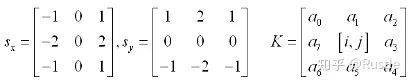
Taking Sobel as an example, where represents the edge detection operator for the X-axis and Y-axis, it can be clearly seen from the operator structure that this filter calculates the difference in grayscale values between the current pixel point and its 8-connected pixels on the left and right. Let’s first understand this through a one-dimensional concept:

For example, we have a one-dimensional array of length 10 with values:

[ 8, 6, 2, 4, 9, 1, 3, 5, 10, 6 ]

At this point, our one-dimensional edge detection operator would be [ -1, 0, 1 ]. Now, we place the edge detection operator over the array to perform a dot product (i.e., the sum of the products of corresponding points), resulting in:

[ 6, -6, -2, 7, -3, -6, 4, 7, 1, -10]

It can be observed that negative values appear in the results, but our previous definition states that the pixel grayscale value is defined within the range of 0-255. Therefore, the usual operation is to truncate negative values to within 0-255 or take the absolute value. Thus, we obtain:

[ 6, 6, 2, 7, 3, 6, 4, 7, 1, 10]

The size of the numbers indicates the magnitude of the gradient at the current pixel point, i.e., how fast the grayscale changes. The larger the value, the more we can be certain that the current point is the edge point we are looking for. Through the one-dimensional example, we can better understand the concept of two-dimensional edge detection, which is to perform two filtering operations along the X-axis and Y-axis, and the resulting values undergo square summation and square root operations to obtain the image gradient at the current pixel point. Let’s understand this process through a diagram:

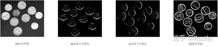
In the figure, (a) is the original grayscale image, (b) and (c) are the filtering results of the original image using the Sobel operator in Figure 3-3, representing the gradient images along the X and Y axes respectively. Finally, combining the two images gives us the required gradient image (d). Here’s another image to help understand the Sobel algorithm:

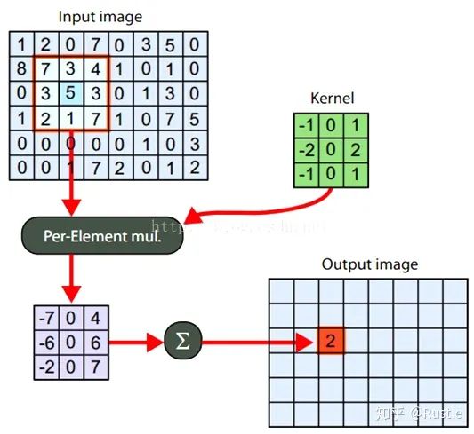
Now we have a general understanding of the basic idea of edge detection. Looking at Figure 3-4(d), isn’t it quite beautiful? However, just because it looks good doesn’t mean it is the edge image we need. The edge image obtained using basic edge operators like Sobel has many issues, such as noise pollution not being eliminated and edges being too thick. Therefore, we will next introduce two advanced edge detection operators: Canny operator and Marr-Hildreth operator.

2. More Advanced Edge Detection Operators

1). Canny Operator

The Canny operator is a multi-stage edge detection algorithm developed by Australian computer scientist John F. Canny in 1986, aimed at finding an optimal edge. The definition of an optimal edge is:

1.Good Detection — The algorithm can mark as many actual edges in the image as possible.

2.Good Localization — The marked edges should be as close as possible to the actual edges in the image.

3.Minimum Response — Edges in the image should only be marked once, and any possible image noise should not be marked as edges.

Next, let’s introduce the specific steps of the popular Canny algorithm.

(1). Gaussian Filtering

Gaussian filtering is currently the most popular denoising filtering algorithm. The term normal in Gaussian refers to the same concept as the normal distribution we learned in probability theory. Its principle is to perform weighted averaging based on the grayscale values of the pixel being filtered and its neighboring points according to the Gaussian formula. This effectively filters out the high-frequency noise added to the ideal image.

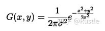
The two-dimensional Gaussian formula is:

Common Gaussian filters include:

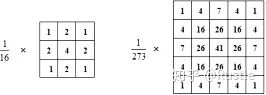
In fact, the Gaussian filter resembles a pyramid structure, where the size of the filter values can be understood as weights. The larger the value, the greater the weight corresponding to the pixel point, and thus the greater the contribution to the grayscale value. Therefore, from the Gaussian filter, we can see that for the current pixel point, the farther away, the smaller the weight, and the smaller the contribution to the grayscale value.

Let’s use an example to understand Gaussian filtering. In the left Gaussian filter of Figure 3-5, we can think of the center point 4 as the ‘main character’, and the surrounding points as ‘neighbors’. The noise can be seen as ‘bad people’. Now, we assume that among these 9 people, one is a ‘bad person’. We also know that bad people will definitely claim to be good people, but what if we have a voting mechanism to decide whether someone is a ‘bad person’? The weights correspond to the weight of each person’s speech, and the voting mechanism is what we call the weighted average strategy. Now we can intuitively see that Gaussian filtering is a filter that considers its surrounding pixel points; even if the current point is a noise point, the Gaussian filter will also constrain the influence of the noise through the grayscale values of the surrounding points.

The code for generating the Gaussian filter and filtering the image is as follows:

sigma=1; % Gaussian standard deviation% Calculate the filter length based on the Gaussian standard deviationfilterExtent = ceil(4*sigma);x = -filterExtent:filterExtent;% Generate one-dimensional Gaussian kernelc = 1/(sqrt(2*pi)*sigma);gaussKernel = c * exp(-(x.^2)/(2*sigma^2));% StandardizationgaussKernel = gaussKernel/sum(gaussKernel);% Perform Gaussian filtering on the image to smoothaSmooth=imfilter(a,gaussKernel,'conv','replicate'); % Convolution along the X-axisaSmooth=imfilter(aSmooth,gaussKernel','conv','replicate'); % Convolution along the Y-axis

(where gaussKernel’ indicates the transposition of gaussKernel)

(2). Calculate Gradient Image and Angle Image

Calculating the gradient image is basically what we have understood so far; it is simply detecting gradients using various edge detection operators. However, the gradient detection operator used in Canny is a bit advanced, as it is derived from the Gaussian filter, and the results are similar to the Sobel operator. The code is as follows:

% Numerical gradient function (1-D derivative of Gaussian kernel)derivGaussKernel = gradient(gaussKernel);% StandardizationnegVals = derivGaussKernel < 0;posVals = derivGaussKernel > 0;derivGaussKernel(posVals) = derivGaussKernel(posVals)/sum(derivGaussKernel(posVals));derivGaussKernel(negVals) = derivGaussKernel(negVals)/abs(sum(derivGaussKernel(negVals)));% Calculate gradientdx = imfilter(aSmooth, derivGaussKernel, 'conv','replicate');dy = imfilter(aSmooth, derivGaussKernel', 'conv','replicate');mag = hypot(dx,dy); magmax = max(mag(:));if magmax>0magGrad = mag / magmax; % Normalize gradientend

The calculation of the angle image is relatively simple, serving as guidance for the direction of non-maximum suppression. The formula is as follows:

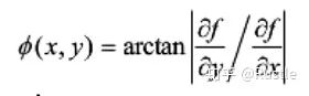
(3). Perform Non-Maximum Suppression on the Gradient Image

The gradient image obtained from the previous step has issues such as thick edges and weak edge interference. Now we can use non-maximum suppression to find the local maxima of pixel points and set the grayscale values corresponding to non-maximum values to 0, thus eliminating a large portion of non-edge pixel points.

As shown in Figure 3-6, C represents the current point of non-maximum suppression, g1-4 are its 8-connected neighboring points, and the blue line segment in the figure indicates the gradient direction value calculated from the angle image at point C. The first step is to check whether the grayscale value of C is the largest among the 8 neighboring values. If so, we then check whether the gradient direction intersection points dTmp1 and dTmp2 are greater than C. If C is greater than the grayscale values of dTmp1 and dTmp2, C is recognized as a maximum value point and set to 1. Therefore, the final generated image should be a binarized image, ideally with edges being single-pixel edges.

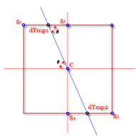
(It is important to note that the gradient direction intersection points do not necessarily fall on the 8 neighboring points; therefore, dTmp1 and dTmp2 are actually the grayscale values formed by bilinear interpolation of the two adjacent points in practical applications.)

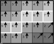
Finally, here’s another image to help everyone understand. As shown in Figure 3-7, the gradient direction is vertically upward. After non-maximum suppression, the maximum value in the gradient direction is taken as the edge point, forming a fine and accurate single-pixel edge.

(4). Use Double Thresholding for Edge Linking

After the above three steps, the quality of the edges obtained is already very high, but there are still many false edges. Therefore, the algorithm used in Canny is double thresholding. The specific idea is to select two thresholds: points below the low threshold are considered false edges and set to 0, points above the high threshold are considered strong edges and set to 1, while pixels in between need further checks.

Based on the high threshold image, edges are linked into contours. When reaching the endpoints of the contour, the algorithm searches among the 8 neighboring points for those satisfying the low threshold, and collects new edges based on this point until the entire image is closed. The specific code is:

function nedge=connect1(nedge,y,x,low,high,magGrad) % Connectivity analysis after seed positioningneighbour=[-1 -1;-1 0;-1 1;0 -1;0 1;1 -1;1 0;1 1]; % 8-connected search[m n]=size(nedge);for k=1:8yy=fix(y+neighbour(k,1));xx=fix(x+neighbour(k,2));if yy>=1 &&yy<=m xx>=1 && xx<=n if magGrad(yy,xx)>=low & nedge(yy,xx)~=255 & magGrad(yy,xx)<high nedge(yy,xx)=255;%disp('check check');%nedge=connect1(nedge,yy,xx,low,high,magGrad);endendendend

However, due to the high computational cost of finding weak edge points because of the recursive thinking, and the number of weak edge points found being few, this step is often omitted in practical applications, replaced by morphological edge thinning operations. The specific idea will be mentioned later, and the specific code is:

H = bwmorph(H, 'thin', 1);

Thus, we have deeply understood the ideas and implementation methods of the Canny algorithm. In practical applications, Canny is generally the first choice for edge detection, and its algorithm ideas are also very worth learning. Next, we will briefly introduce the Marr-Hildreth edge detection operator based on second-order derivatives.

1). Marr-Hildreth Operator

Before learning the Marr-Hildreth operator, let’s first understand why we need to use second-order derivatives.

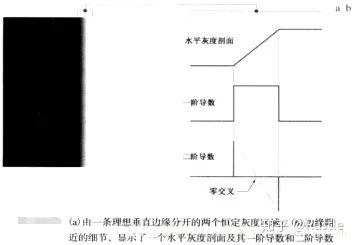
As shown in Figure 3-8, the left side represents a grayscale image that gradually changes from black (0) to white (255) from left to right. Now let’s look at its horizontal grayscale profile; the grayscale value rises steadily from low to high, and its first derivative is represented by a constant value in the rising area, where the information obtained is that the grayscale value of the image transitions smoothly, i.e., the gradient value is equal. Next, when we take its second derivative, we find that at the starting transition point, it is positive, and its value is the gradient value of the first derivative at this point. The ending point is also like the starting point. Now, the key point is that if we connect these two points, we obtain a crossing point with the X-axis, which is considered an edge point. This is the wonderful application of second-order derivatives in the field of edge detection (I found it amazing when I first encountered it).

Let’s look at the conclusions of Marr and Hildreth:

1. Grayscale changes are independent of image size, so their detection requires operators of different sizes.

2. Sudden changes in grayscale will cause peaks or valleys in the first derivative, which equivalently cause zero crossings in the second derivative.

After learning the principle of the Marr-Hildreth algorithm based on second-order derivatives, let’s look at its approach:

(1). Gaussian Filtering

You read that right, it’s still Gaussian filtering. Almost all edge detection algorithms will add a Gaussian filter to remove high-frequency noise, so there’s no need to elaborate further; just review the previous sections.

(2). Calculate Laplacian Second Derivative

Marr-Hildreth proves that the filter Laplacian of Gaussian (LoG) is the most suitable operator for image processing needs. We will not elaborate on the specific principles here; let’s look at its formula:

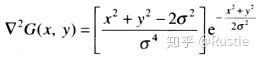
The generated Laplacian filter is also known as the Mexican Hat Operator, because its center is generally a larger positive number, while the 8-connected neighboring points have smaller negative values. Common filters are shown in Figure 3-9:

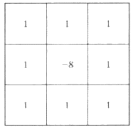
Next, we perform filtering operations on the image using the Laplacian filter to obtain the image to be calculated.

(3). Calculate Zero Crossing

Zero crossing is relatively simple to implement. Since zero crossing points indicate that at least two adjacent pixel points have opposite signs, there are four situations to detect: left and right, up and down, and two diagonals. If the absolute difference of any of the four situations at pixel p in the filtered image g(x, y) exceeds the set threshold, we can call p a zero crossing pixel, as illustrated below:

This is a small part of Marr-Hildreth, checking whether the condition [ – +] is satisfied, where thresh is the aforementioned threshold.

By now, we have learned about two of the most popular and classic advanced edge detection algorithms and ideas. Next, we will discuss some experiences and algorithm selection references.

4. Supplement

1. The size of the filter should be odd, so that there is a center point for assignment operations. Common filters or convolution kernels (Conv kernel) include 3*3, 5*5, etc., hence the concept of radius, for example, a 5*5 convolution kernel has a radius of 2.

2. The sum of all elements in the filter should be 0; this constraint ensures that the overall grayscale value of the image remains unchanged before and after filtering.

3. The Roberts operator, Sobel operator, and Prewitt operator have high operational speeds and certain suppression of noise, but the quality of the detected edges is not high, such as thick edges, inaccurate localization, and many discontinuities.

4. The Canny operator is not easily affected by noise, yielding fine and accurate edges. The downside is that the computational cost is high, making it difficult to run in real-time image processing; it is suitable for applications requiring high precision.

5. The Marr-Hildreth operator has relatively good edge detection effects but is sensitive to noise (due to the nature of its second-order operations).

5. Conclusion

Overall, edge detection algorithms have a wide range of applications across many fields and are an excellent entry point for learning Computer Vision. Many ideas and principles from these algorithms still resonate with me. Therefore, I thought it would be a good start to write my first article on this topic. Additionally, some parts of the article reflect my own understanding and insights; if there are any errors, I hope everyone can point them out. I will continue to write articles on Machine Learning, Deep Learning, and Face Recognition. Finally, I will attach the complete Matlab code implementation of the Canny edge detection algorithm (of course, you can also call the edge function, but for learning purposes, it’s best to implement it from the ground up).

I=imread('cameraman.tif');%I=rgb2gray(I);figure(1);subplot(121);imshow(I);xlabel('Original Image');[m n]=size(I);a=double(I);sigma=1; % Gaussian standard deviation%highThresh=0.0625; % Upper threshold%lowThresh=0.0250 ; % Lower threshold%=======================Gaussian Filtering & Gradient Calculation=======================%%%%%%%%%%%%%%%%%%%%%%%%%Old%%%%%%%%%%%%%%%%%%%%%%%%%%%%pw = 1:30; %ssq = sigma^2;%width = find(exp(-(pw.*pw)/(2*ssq))>0.0001,1,'last');%if isempty(width)% width = 1; %end%t = (-width:width);%gauss = exp(-(t.*t)/(2*ssq))/(2*pi*ssq); % One-dimensional Gaussian filter%[x,y]=meshgrid(-width:width,-width:width);%gauss2=-x.*exp(-(x.*x+y.*y)/(2*ssq))/(pi*ssq); % Two-dimensional Gaussian filter%Perform Gaussian filtering on the image to smooth%aSmooth=imfilter(a,gauss,'conv','replicate'); % Convolution along the X-axis%aSmooth=imfilter(aSmooth,gauss','conv','replicate'); % Convolution along the Y-axis%=============================================== Calculate filter length based on Gaussian standard deviationfilterExtent = ceil(4*sigma);x = -filterExtent:filterExtent;% Generate one-dimensional Gaussian kernelc = 1/(sqrt(2*pi)*sigma);gaussKernel = c * exp(-(x.^2)/(2*sigma^2));% StandardizationgaussKernel = gaussKernel/sum(gaussKernel);% Numerical gradient function (1-D derivative of Gaussian kernel)derivGaussKernel = gradient(gaussKernel);% StandardizationnegVals = derivGaussKernel < 0;posVals = derivGaussKernel > 0;derivGaussKernel(posVals) = derivGaussKernel(posVals)/sum(derivGaussKernel(posVals));derivGaussKernel(negVals) = derivGaussKernel(negVals)/abs(sum(derivGaussKernel(negVals)));% Perform Gaussian filtering on the image to smoothaSmooth=imfilter(a,gaussKernel,'conv','replicate'); % Convolution along the X-axisaSmooth=imfilter(aSmooth,gaussKernel','conv','replicate'); % Convolution along the Y-axis%hv=fspecial('sobel');% Calculate gradientdx = imfilter(aSmooth, derivGaussKernel, 'conv','replicate');dy = imfilter(aSmooth, derivGaussKernel', 'conv','replicate');mag = hypot(dx,dy); magmax = max(mag(:));if magmax>0magGrad = mag / magmax; % Normalize gradientend% Threshold selection%PercentOfPixelsNotEdges = 0.7; counts=imhist(magGrad, 64);highThresh = find(cumsum(counts) > 0.7*m*n, 1 ,'first' ) / 64;lowThresh = 0.4*highThresh;%figure(8);imshow(magGrad);%%========================Gaussian Filtering========================================%w=fspecial('gaussian',[5 5]);%img=imfilter(img,w,'replicate');%figure;%imshow(uint8(img))%%===================Sobel Edge Detection=======================================%hv=fspecial('sobel');%dx=imfilter(img,hv,'replicate'); % Calculate horizontal edges%hh=hv';%dy=imfilter(img,hh,'replicate'); % Calculate vertical edges%img=sqrt(dx.^2+dy.^2); % magmax = max(img(:));% (Threshold selection normalization)% if magmax > 0% magGrad = img / magmax;% end%figure;%imshow(uint8(img));I = thinAndThreshold(dx, dy, magGrad, lowThresh, highThresh);%disp(lowThresh);subplot(122);imshow(I);xlabel('Canny Edge Detection');disp("High Threshold TL: " + highThresh);disp("Low Threshold TH: " + lowThresh);%========================Non-Maximum Suppression and Edge Linking=======================================function H = thinAndThreshold(dx, dy, magGrad, lowThresh, highThresh)E = cannyFindLocalMaxima(dx,dy,magGrad,lowThresh); % Non-maximum suppressionif ~isempty(E)[rstrong,cstrong] = find(magGrad>highThresh & E);if ~isempty(rstrong) H = bwselect(E, cstrong, rstrong, 8); % Select strong edges in 8-connected targets% figure(2);imshow(H);% set(0,'RecursionLimit',1000); % Weak edge connectivity (not very useful, and computation time is long)% [xstrong ystrong]=find(magGrad>highThresh & E);% for i=1:numel(xstrong);% H = connect1(H,xstrong(i),ystrong(i),lowThresh,highThresh,magGrad);% end% figure(3);imshow(H);H = bwmorph(H, 'thin', 1); % Edge thinningelseH = false(size(E));endelseH = false(size(E));endend%========================Weak Edge Linking=======================================function nedge=connect1(nedge,y,x,low,high,magGrad) % Connectivity analysis after seed positioningneighbour=[-1 -1;-1 0;-1 1;0 -1;0 1;1 -1;1 0;1 1]; % 8-connected search[m n]=size(nedge);for k=1:8yy=fix(y+neighbour(k,1));xx=fix(x+neighbour(k,2));if yy>=1 &&yy<=m xx>=1 && xx<=n if magGrad(yy,xx)>=low & nedge(yy,xx)~=255 &>=high nedge(yy,xx)=255;%disp('check check');%nedge=connect1(nedge,yy,xx,low,high,magGrad);endendendend

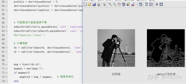
The effects are shown in the figure:

Summary of Highlights in This Article

1.Edge detection algorithms aim to find an optimal edge, defined as:

1. Good Detection — The algorithm should mark as many actual edges in the image as possible.

2. Good Localization — The marked edges should be as close as possible to the actual edges in the image.

3. Minimum Response — Edges in the image should only be marked once, and any possible image noise should not be marked as edges.

2.Gaussian filtering is currently the most popular denoising algorithm. The term normal in Gaussian refers to the same concept as the normal distribution we learned in probability theory, where the principle is to perform weighted averaging based on the grayscale values of the pixel being filtered and its neighboring points according to the Gaussian formula, effectively filtering out the high-frequency noise added to the ideal image.

Good news!
Xiaobai Learns Vision Knowledge Planet
Is now open to the public👇👇👇



Download 1: OpenCV-Contrib Extension Module Chinese Version Tutorial
Reply "Extension Module Chinese Tutorial" in the background of the "Xiaobai Learns Vision" public account to download the first OpenCV extension module tutorial in Chinese, covering installation of extension modules, SFM algorithms, stereo vision, target tracking, biological vision, super-resolution processing, and more than twenty chapters of content.

Download 2: Python Vision Practical Project 52 Lectures
Reply "Python Vision Practical Projects" in the background of the "Xiaobai Learns Vision" public account to download 31 practical projects including image segmentation, mask detection, lane line detection, vehicle counting, eyeliner addition, license plate recognition, character recognition, emotion detection, text content extraction, and face recognition, helping to quickly learn computer vision.

Download 3: OpenCV Practical Project 20 Lectures
Reply "OpenCV Practical Project 20 Lectures" in the background of the "Xiaobai Learns Vision" public account to download 20 practical projects based on OpenCV implementation, achieving advanced OpenCV learning.

Group Chat

You are welcome to join the reader group of the public account to communicate with peers. Currently, there are WeChat groups for SLAM, 3D vision, sensors, autonomous driving, computational photography, detection, segmentation, recognition, medical imaging, GAN, algorithm competitions, etc. (will be gradually subdivided in the future). Please scan the WeChat ID below to join the group, with the note: "Nickname + School/Company + Research Direction", for example: "Zhang San + Shanghai Jiao Tong University + Vision SLAM". Please follow the format for notes; otherwise, you will not be approved. After successful addition, you will be invited to relevant WeChat groups based on your research direction. Please do not send advertisements in the group; otherwise, you will be removed from the group. Thank you for your understanding~