There is something that might surprise beginners:Neural network models are not complex!The term ‘neural network’ sounds impressive, but in reality, neural network algorithms are simpler than people think.
This article is entirely prepared for beginners. We will understand the principles of neural networks by implementing a neural network from scratch using Python. The outline of this article is as follows:
- Introduction to the basic structure of neural networks – neurons;
- Using the sigmoid activation function in neurons;
- A neural network is a collection of connected neurons;
- Constructing a dataset where the inputs (or features) are weight and height, and the output (or label) is gender;
- Learning about loss functions and mean squared error loss;
- Training the network means minimizing its loss;
- Calculating partial derivatives using backpropagation;
- Training the network using stochastic gradient descent.

Block: Neuron

First, let’s take a look at the basic unit of a neural network, the neuron.The neuron accepts inputs, performs some data operations on them, and then produces outputs.For example, here is a 2-input neuron:
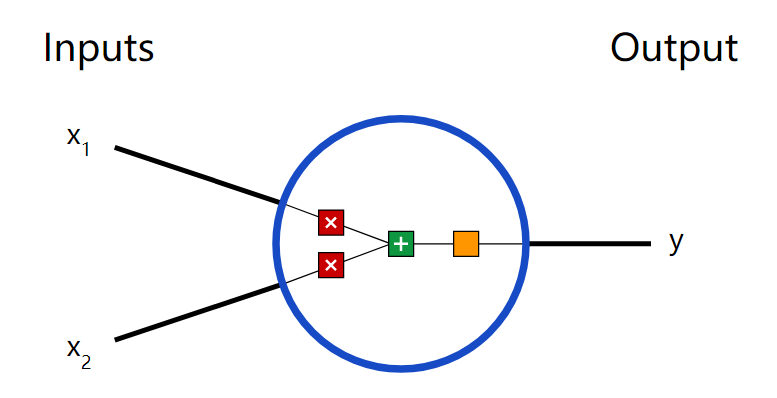
Three things happen here. First, each input is multiplied by a weight (red):
Then, the weighted inputs are summed up and a bias b (green) is added:
Finally, this result is passed to an activation function f:
The purpose of the activation function is to transform an unbounded input into a predictable form. A commonly used activation function is the sigmoid function:
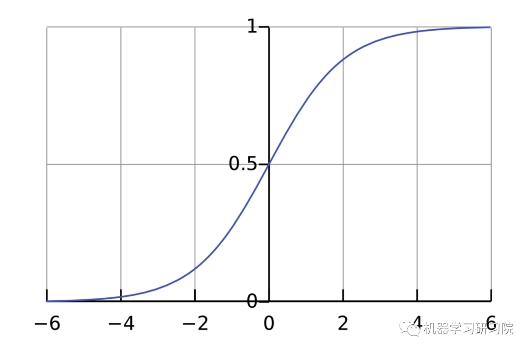
The range of the sigmoid function is (0, 1). In simple terms, it compresses (−∞, +∞) to (0, 1), where large negative numbers are approximately 0 and large positive numbers are approximately 1.
A simple example
Suppose we have a neuron with the sigmoid activation function and the following parameters:
It is represented in vector form. Now, we give this neuron an input. We express it using the dot product:
When the input is [2, 3], the output of this neuron is 0.999. The process of obtaining the output given the input is called feedforward.
Coding a neuron
Let’s implement a neuron! We will use the NumPy library in Python to perform the mathematical calculations:
<pre><code class="language-python">import numpy as np

def sigmoid(x):

    # Our activation function: f(x) = 1 / (1 + e^(-x))

    return 1 / (1 + np.exp(-x))
class Neuron:
def __init__(self, weights, bias):
self.weights = weights
self.bias = bias
def feedforward(self, inputs):
# Weighted input, add bias, then use activation function
total = np.dot(self.weights, inputs) + self.bias
return sigmoid(total)
weights = np.array([0, 1]) # w1 = 0, w2 = 1
bias = 4 # b = 4
n = Neuron(weights, bias)
x = np.array([2, 3]) # x1 = 2, x2 = 3
print(n.feedforward(x)) # 0.9990889488055994
Do you remember this number? It is the 0.999 we calculated in the previous example.
Assembling neurons into a network
The so-called neural network is a collection of neurons. Here is a simple neural network:
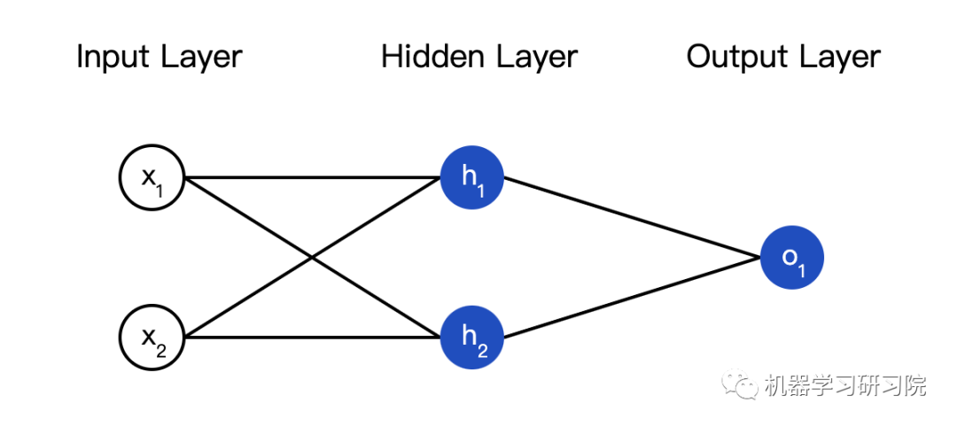
This network has two inputs, a hidden layer with two neurons (h1, h2), and an output layer with one neuron (o1). Note that the input to o1 is the output from h1 and h2, thus forming a network.
The hidden layer is the layer between the input layer and the output layer, and there can be multiple hidden layers.
Example: Feedforward
Continuing with the network from the previous diagram, suppose each neuron’s weights are and the intercept is the same with the activation function also being the sigmoid function.Let’s denote the corresponding neuron outputs as .
What result do we get when the input is ?
The output of this neural network for the input is 0.7216, which is quite simple.
The number of layers in a neural network and the number of neurons in each layer can be arbitrary. The basic logic remains the same: inputs are transmitted forward through the neural network, ultimately yielding outputs. Next, we will continue using this network.
Coding the neural network: Feedforward
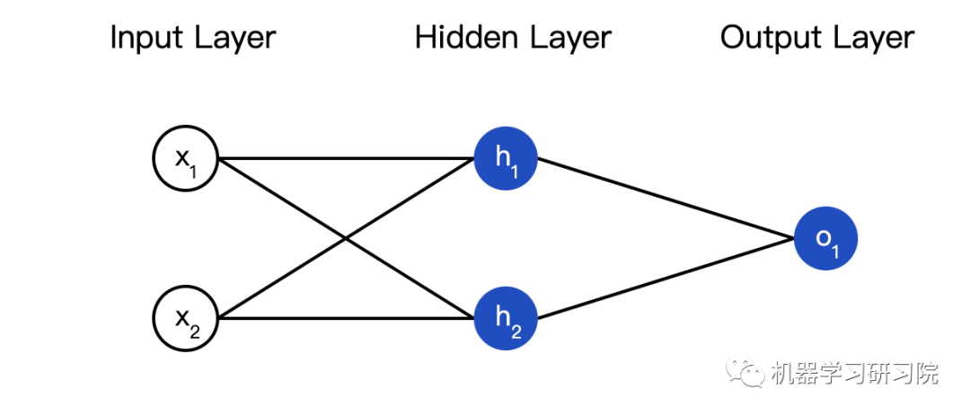
Next, we will implement the feedforward mechanism of this neural network, using the same diagram:
<pre><code class="language-python">import numpy as np

# ... code from previous section here

class OurNeuralNetwork:

    '''  A neural network with:

    - 2 inputs

    - a hidden layer with 2 neurons (h1, h2)

    - an output layer with 1 neuron (o1)

    Each neuron has the same weights and bias:

    - w = [0, 1]

    - b = 0

    '''

    def __init__(self):

        weights = np.array([0, 1])

        bias = 0

        # Here is the neuron class from the previous section

        self.h1 = Neuron(weights, bias)

        self.h2 = Neuron(weights, bias)

        self.o1 = Neuron(weights, bias)
def feedforward(self, x):
out_h1 = self.h1.feedforward(x)
out_h2 = self.h2.feedforward(x)
# The input to o1 is the output from h1 and h2
out_o1 = self.o1.feedforward(np.array([out_h1, out_h2]))
return out_o1
network = OurNeuralNetwork()
x = np.array([2, 3])
print(network.feedforward(x)) # 0.7216325609518421
The result is correct, everything looks good.
Training the Neural Network Part 1
Now we have the following data:
| Name | Weight (lbs) | Height (inches) | Gender |
|---|---|---|---|
| Alice | 133 | 65 | F |
| Bob | 160 | 72 | M |
| Charlie | 152 | 70 | M |
| Diana | 120 | 60 | F |
Next, we will use this data to train the weights and intercepts of the neural network so that it can predict gender based on height and weight:
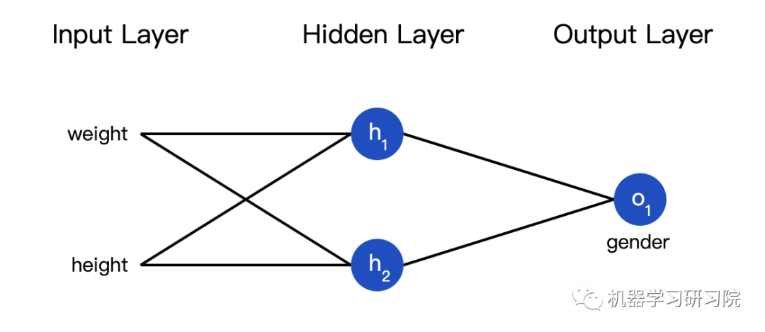
We will represent males (M) and females (F) as 0 and 1, respectively, and have transformed the values:
| Name | Weight (subtract 135) | Height (subtract 66) | Gender |
|---|---|---|---|
| Alice | -2 | -1 | 1 |
| Bob | 25 | 6 | 0 |
| Charlie | 17 | 4 | 0 |
| Diana | -15 | -6 | 1 |
I randomly chose 135 and 66 to normalize the data; typically, the mean value is used.
Loss
Before training the network, we need to quantify whether the current network is ‘good’ or ‘bad’ so that we can look for a better network.This is the purpose of defining loss.
Here we use the Mean Squared Error (MSE) loss: , let’s take a closer look:
- is the number of samples, which is 4 here (Alice, Bob, Charlie, and Diana).
- represents the variable to be predicted, which is gender here.
- is the true value of the variable (‘correct answer’). For example, Alice’s is 1 (female).
- is the predicted value of the variable. This is the output of our network.
is known as the squared error. Our loss function is the average of all squared errors. The better the prediction, the less the loss.
Better predictions = Less loss!
Training the network = Minimizing its loss.
Example of loss calculation
Suppose our network always outputs 0, in other words, it thinks everyone is male. What is the loss?
| Name | y_true | y_pred | (y_true – y_pred)^2 |
|---|---|---|---|
| Alice | 1 | 0 | 1 |
| Bob | 0 | 0 | 0 |
| Charlie | 0 | 0 | 0 |
| Diana | 1 | 0 | 1 |
Code: MSE loss
Here is the code to calculate MSE loss:
<pre><code class="language-python">import numpy as np

def mse_loss(y_true, y_pred):

    # y_true and y_pred are numpy arrays of the same length.

    return ((y_true - y_pred) ** 2).mean()

y_true = np.array([1, 0, 0, 1])

y_pred = np.array([0, 0, 0, 0])

print(mse_loss(y_true, y_pred))  # 0.5
If you don’t understand this code, you can refer to the quick start on NumPy regarding array operations.
Alright, let’s continue.
Training the Neural Network Part 2
Now we have a clear goal: minimize the loss of the neural network. By adjusting the weights and intercepts of the network, we can change its prediction results, but how can we gradually reduce the loss?
This section involves multivariable calculus; if you are not familiar with calculus, you can skip this mathematical content.
To simplify the problem, let’s assume we only have Alice in our dataset:
Suppose our network always outputs 0, which means it thinks everyone is male. What is the loss?
| Name | Weight (subtract 135) | Height (subtract 66) | Gender |
|---|---|---|---|
| Alice | -2 | -1 | 1 |
Then the mean squared error loss is just Alice’s squared error:
We can also view the loss as a function of weights and intercepts. Let’s label the network with weights and intercepts:
Thus, we can express the network’s loss as:
Assuming we want to optimize , how will the loss change when we alter ? We can answer this question using , how to calculate it?
The following data is a bit complex; don’t worry, prepare some paper and a pen.
First, let’s rewrite this partial derivative:
Since we already know , we can calculate
Now let’s deal with . They represent the outputs of the respective neurons, and we have:
Since only will affect (not ), we have:
Here, is height, and is weight. This is the second time we see .
We will use this later.
Got it! This result means that increasing will also slightly increase.
Training: Stochastic Gradient Descent
Now everything is ready to train the neural network! We will use an optimization algorithm called stochastic gradient descent to optimize the weights and intercepts of the network, minimizing the loss. The core is this update equation:
is a constant known as the learning rate, which adjusts the speed of training. What we need to do is subtract from :
- If is positive, will decrease, will go down.
- If is negative, will increase, will go up.
If we optimize each weight and intercept in the network this way, the loss will continuously decrease, and the network’s performance will improve.
Our training process is as follows:
- Select a sample from our dataset and optimize using stochastic gradient descent – we optimize one sample at a time;
- Calculate the partial derivative of each weight or intercept (e.g., , etc.);
- Update each weight and intercept using the update equation;
- Repeat the first step;
Code: A Complete Neural Network
We can finally implement a complete neural network:
| Name | Height (subtract 135) | Weight (subtract 66) | Gender |
|---|---|---|---|
| Alice | -2 | -1 | 1 |
| Bob | 25 | 6 | 0 |
| Charlie | 17 | 4 | 0 |
| Diana | -15 | -6 | 1 |
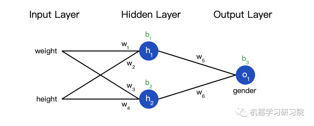
<pre><code class="language-python">import numpy as np

def sigmoid(x):

    # Sigmoid activation function: f(x) = 1 / (1 + e^(-x))

    return 1 / (1 + np.exp(-x))
def deriv_sigmoid(x):
# Derivative of sigmoid: f'(x) = f(x) * (1 - f(x))
fx = sigmoid(x)
return fx * (1 - fx)
def mse_loss(y_true, y_pred):
# y_true and y_pred are numpy arrays of the same length.
return ((y_true - y_pred) ** 2).mean()
class OurNeuralNetwork:
''' A neural network with:
- 2 inputs
- a hidden layer with 2 neurons (h1, h2)
- an output layer with 1 neuron (o1)
*** Disclaimer ***: The following code is for simplicity and demonstration purposes, not optimal.
Real neural network code is completely different. Do not use this code. Instead, read/run it to understand how this specific network works. '''
def __init__(self):
# Weights
self.w1 = np.random.normal()
self.w2 = np.random.normal()
self.w3 = np.random.normal()
self.w4 = np.random.normal()
self.w5 = np.random.normal()
self.w6 = np.random.normal()
# Biases
self.b1 = np.random.normal()
self.b2 = np.random.normal()
self.b3 = np.random.normal()
def feedforward(self, x):
# X is an array of numbers with 2 elements.
h1 = sigmoid(self.w1 * x[0] + self.w2 * x[1] + self.b1)
h2 = sigmoid(self.w3 * x[0] + self.w4 * x[1] + self.b2)
o1 = sigmoid(self.w5 * h1 + self.w6 * h2 + self.b3)
return o1
def train(self, data, all_y_trues):
'''
- data is a (n x 2) numpy array, n = # of samples in the dataset.
- all_y_trues is a numpy array with n elements.
Elements in all_y_trues correspond to those in data.
'''
learn_rate = 0.1
epochs = 1000 # Number of times to iterate through the dataset
for epoch in range(epochs):
for x, y_true in zip(data, all_y_trues):
# --- Do a feedforward (we will need these values later)
sum_h1 = self.w1 * x[0] + self.w2 * x[1] + self.b1
h1 = sigmoid(sum_h1)
sum_h2 = self.w3 * x[0] + self.w4 * x[1] + self.b2
h2 = sigmoid(sum_h2)
sum_o1 = self.w5 * h1 + self.w6 * h2 + self.b3
o1 = sigmoid(sum_o1)
y_pred = o1
# --- Calculate partial derivatives.
# --- Naming: d_L_d_w1 represents "partial L / partial w1"
d_L_d_ypred = -2 * (y_true - y_pred)
# Neuron o1
d_ypred_d_w5 = h1 * deriv_sigmoid(sum_o1)
d_ypred_d_w6 = h2 * deriv_sigmoid(sum_o1)
d_ypred_d_b3 = deriv_sigmoid(sum_o1)
d_ypred_d_h1 = self.w5 * deriv_sigmoid(sum_o1)
d_ypred_d_h2 = self.w6 * deriv_sigmoid(sum_o1)
# Neuron h1
d_h1_d_w1 = x[0] * deriv_sigmoid(sum_h1)
d_h1_d_w2 = x[1] * deriv_sigmoid(sum_h1)
d_h1_d_b1 = deriv_sigmoid(sum_h1)
# Neuron h2
d_h2_d_w3 = x[0] * deriv_sigmoid(sum_h2)
d_h2_d_w4 = x[1] * deriv_sigmoid(sum_h2)
d_h2_d_b2 = deriv_sigmoid(sum_h2)
# --- Update weights and biases
# Neuron h1
self.w1 -= learn_rate * d_L_d_ypred * d_ypred_d_h1 * d_h1_d_w1
self.w2 -= learn_rate * d_L_d_ypred * d_ypred_d_h1 * d_h1_d_w2
self.b1 -= learn_rate * d_L_d_ypred * d_ypred_d_h1 * d_h1_d_b1
# Neuron h2
self.w3 -= learn_rate * d_L_d_ypred * d_ypred_d_h2 * d_h2_d_w3
self.w4 -= learn_rate * d_L_d_ypred * d_ypred_d_h2 * d_h2_d_w4
self.b2 -= learn_rate * d_L_d_ypred * d_ypred_d_h2 * d_h2_d_b2
# Neuron o1
self.w5 -= learn_rate * d_L_d_ypred * d_ypred_d_w5
self.w6 -= learn_rate * d_L_d_ypred * d_ypred_d_w6
self.b3 -= learn_rate * d_L_d_ypred * d_ypred_d_b3
# --- Calculate total loss at the end of each epoch
if epoch % 10 == 0:
y_preds = np.apply_along_axis(self.feedforward, 1, data)
loss = mse_loss(all_y_trues, y_preds)
print("Epoch %d loss: %.3f" % (epoch, loss))
# Define dataset
data = np.array([
[-2, -1], # Alice
[25, 6], # Bob
[17, 4], # Charlie
[-15, -6], # Diana
])
all_y_trues = np.array([
1, # Alice
0, # Bob
0, # Charlie
1, # Diana
])
# Train our neural network!
network = OurNeuralNetwork()
network.train(data, all_y_trues)
As the network learns, the loss steadily decreases.
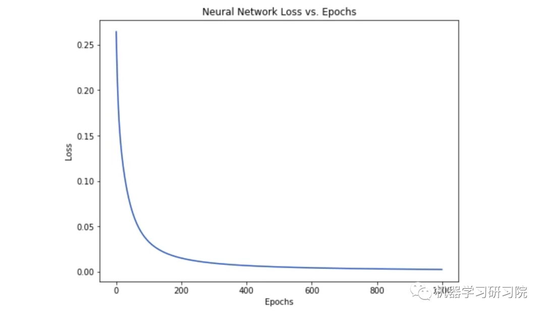
Now we can use this network to predict gender:
<pre><code class="language-python"># Make some predictions

emily = np.array([-7, -3])  # 128 lbs, 63 inches

frank = np.array([20, 2])    # 155 lbs, 68 inches

print("Emily: %.3f" % network.feedforward(emily))  # 0.951 - F

print("Frank: %.3f" % network.feedforward(frank))  # 0.039 - M
What’s next?
We have completed a simple neural network. Let’s quickly review:
- Introduced the basic structure of neural networks – neurons;
- Used the sigmoid activation function in neurons;
- A neural network is a collection of connected neurons;
- Constructed a dataset where the inputs (or features) are weight and height, and the output (or label) is gender;
- Learned about loss functions and mean squared error loss;
- Training a network means minimizing its loss;
- Calculated partial derivatives using backpropagation;
- Trained the network using stochastic gradient descent;
Next, you can:
- Implement larger and better neural networks using machine learning libraries such as TensorFlow, Keras, and PyTorch;
- Explore other types of activation functions;
- Investigate other types of optimizers;
- Learn about convolutional neural networks, which have revolutionized the field of computer vision;
- Study recurrent neural networks, commonly used in natural language processing;
Author: Victor ZhouOriginal link: https://victorzhou.com/blog/intro-to-neural-networks/

END
Editor / Fan Ruqiang
Reviewer / Fan Ruqiang
Recheck / Fan Ruqiang
Click below
Follow us